\(\renewcommand\AA{\text{Å}}\)

18. GSASIIscriptable: Scripting Interface

18.1. Summary/Contents

GSASIIscriptable provides routines to use an increasing amount of GSAS-II’s capabilities from Python scripts, without use of the graphical user interface (GUI). GSASIIscriptable can create and access GSAS-II project (.gpx) files and can directly perform image handling, peak fits, refinements… The .gpx files are completely compatible with the GUI, so one can move back and forth between the GUI and scripting when developing scripts. This mode of code development is encouraged to get started with GSAS-II scripting.

GSASIIscriptable is normally used by writing Python commands via this module’s application programming interface (API). (There is also an older mechanism where GSASIIscriptable can be accessed via shell/batch commands, see GSASIIscriptable Command-line Interface, called command-line mode.) Access to GSASIIscriptable via the API is used more widely than via command-line mode and offers many more features. The material below introduces and summarizes use of GSASIIscriptable via the API. Following that, detailed descriptions of all routines are provided in the complete API documentation section.

While the command-line mode provides access a number of features without writing Python scripts via shell/batch commands (see GSASIIscriptable Command-line Interface), use in practice seems somewhat clumsy. Command-line mode is no longer being developed and its use is discouraged.

GSASIIscriptable is designed around the hierarchical structure of .gpx files, that is seen in the GUI as the GSAS-II data tree. The module defines wrapper classes (inheriting from G2ObjectWrapper) for most GSAS-II data tree items, so most scripting is done with object-oriented code that operate on different types of data tree objects. At the top level one has a project (G2Project) which contains phases (G2Phase) powder diffraction histograms ( G2PwdrData).

18.2. Installation of GSASIIscriptable

GSASIIscriptable is included as part of a standard GSAS-II installation that includes the GSAS-II GUI (as described in the installation instructions). People who will will use scripting extensively will still need access to the GUI for some activities, since the scripting API does not cover all features of GSAS-II. Even if that were to be completed, there will still be some things that GSAS-II does with the GUI would be almost impossible to implement without a interactive graphical view of the project.

Nonetheless, there may be times where it does make sense to install GSAS-II without all of the Python packages needed for running the GUI, for example on a compute server or cluster. The minimal requirements for use of GSASIIscriptable are:

python

numpy

scipy

GSASIIscriptable can be used without these packages, but with significantly reduced functionality, so their inclusion is highly recommended:

PyCifRW

requests

There are a few other packages that may be used in GSASIIscriptable, for example to import specific types of powder or image data or perform specific types of computations. They are not commonly needed, but if access is attempted, it should be obvious from error messages:

h5py

xmltodict

pybaselines

seekpath

matplotlib

pillow

More information on Python packages used in GSAS-II is provided in the Scripting Requirements section of the Requirements chapter, which also provides some installation instructions.

18.3. Accessing the GSASIIscriptable Module

When GSAS-II is installed with GSAS2MAIN or GSAS2PKG, or with the gitstrap.py script, or directly with git, the GSAS-II software is installed outside of Python. When the GUI is invoked, a small script or Windows batch file is used to invoke Python with a reference to a file (named G2.py) that starts the GSAS-II GUI. It is also possible to install GSAS-II inside Python (for example with pixi), but work on this is not yet complete or documented.

When GSASIIscriptable is used, and GSAS-II has been installed outside of Python, some mechanism is needed to provide the location of the GSAS-II files. There are two ways this can be done:

define the GSAS-II installation location in the Python sys.path, or

install a reference to GSAS-II inside the Python installation.

The latter method requires an extra installation step, but has the advantage that it allows writing portable GSAS-II scripts.

18.3.1. Explicit GSASIIscriptable Specification

MacOS/Linux:

The example below is for MacOS/Linux and assumes that GSAS-II has been installed in location /Users/toby/g2main/ such that there is a directory /Users/toby/g2main/GSAS-II/GSASII that contains all the GSAS-II Python files such as GSASIIscriptable.py. Place code like this into the beginning of your script so that the location of GSAS-II files can be found:
import sys
sys.path.insert(0,'/Users/toby/g2main/GSAS-II') # needed to find GSASII package
from GSASII import GSASIIscriptable as G2sc

Windows:

A similar example, but for Windows, assumes that GSAS-II has been installed in location C:\Users\toby\gsas2main such that there is a directory C:\Users\toby\gsas2main\GSAS-II\GSASII that contains all the GSAS-II Python files such as GSASIIscriptable.py. Place code like this into the beginning of your script (note that use of forward slashes is deliberate; to use back slashes, they must be doubled or placed in a raw-string, 'C:\\Users\\...' or r'C:\Users\...'):
import sys
sys.path.insert(0,'/Users/toby/gsas2main/GSAS-II') # needed to find GSASII package
from GSASII import GSASIIscriptable as G2sc
Note that the directory that is placed in the path is the one that contains the GSASII directory. Previously, this path contained this directory, but now is its parent.

18.3.2. Install GSASIIscriptable Location Into Python

As an alternative to defining the location of GSAS-II in every script, you can define the location of GSAS-II inside Python once, but note that this must be done for each version of Python, if you plan to use GSAS-II scripting with more that one. If you have more than one version of GSAS-II installed, only one can be defined for a Python installation, but the previous method, where sys.path is modified, can be used with all of the GSAS-II installions.

There are three different ways to use GSAS-II to define a location for GSASIIscriptable. You can choose the method that is easiest for you.
The most easy option is to invoke the “Install GSASIIscriptable shortcut” command in the GSAS-II GUI File menu.

This performs the same actions as below, but since the location of both Python and the GSAS-II files are defined within the GUI, no additional input is needed.
Alternatively, using the commands modeled after the ones above, add the Python command G2sc.installScriptingShortcut() into your script as:
import sys
sys.path.insert(0,'/Users/toby/gsas2main/GSAS-II') # needed to find GSASII package
from GSASII import GSASIIscriptable as G2sc
G2sc.installScriptingShortcut()
This only needs to be done once. After the script has been run, remove the command or comment it out.
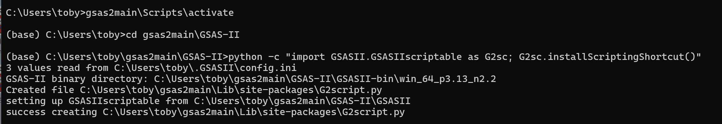
The third choice is to run two command-line (bash/zsh/DOS,…) commands. This assumes that the intended Python interpreter is already in the path. (If not use a conda activate command.) Note that the directory that is used is the parent of the GSASII directory (the directory that contains GSASII.)

Here are the commands on MacOS/Linux:
% cd /Users/toby/gsas2main/GSAS-II
% python -c "import GSASII.GSASIIscriptable as G2sc; G2sc.installScriptingShortcut()"
On Windows the commands in a cmd.exe window will be similar:
>cd \Users\toby\gsas2main\GSAS-II
>python -c "import GSASII.GSASIIscriptable as G2sc; G2sc.installScriptingShortcut()"
The output from this process on Windows is shown below.
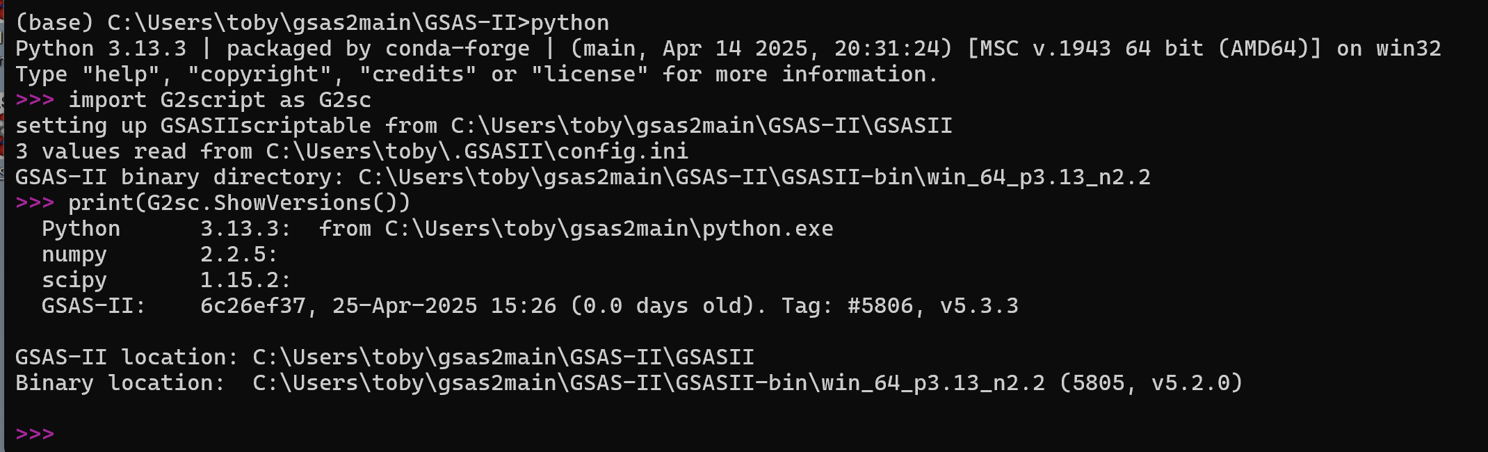
Once any of the above three choices has been completed, a good test to see if GSASIIscriptable is working will be commands:
import G2script as G2sc
print(G2sc.ShowVersions())
as is shown in the image below.

18.3.3. When GSAS-II is Installed Inside Python

If GSAS-II is installed inside of Python, the location of the GSAS-II software is established without any changes to the path so this command should work without using any of the above:
from GSASII import GSASIIscriptable as G2sc

18.4. Application Interface (API) Summary

This section of the documentation provides an overview to API, with full documentation in the API: Complete Documentation section. The typical API use will be with a Python script, such as what is found in Code Examples. Most functionality is provided via the objects and methods summarized below.

18.4.1. Overview of Classes

Scripting class name	Description
G2Project	`G2Project`: A GSAS-II project file; provides references to objects below, each corresponding to a tree item (exception is `G2AtomRecord`)
G2Phase	`G2Phase`: Provides phase information access (also provides access to atom info via `G2AtomRecord`)
G2AtomRecord	`G2AtomRecord`: Access to an atom within a phase
G2PwdrData	`G2PwdrData`: Access to powder histogram info
G2Single	`G2Single`: Access to single crystal histogram info
G2Image	`G2Image`: Access to image info
G2PDF	`G2PDF`: PDF histogram info
G2SmallAngle	`G2SmallAngle`: Small Angle scattering histogram info
G2SeqRefRes	`G2SeqRefRes`: The sequential results table

18.4.2. Independent Functions

A small number of Scriptable routines do not require existence of a G2Project object.

method	Use
`ShowVersions()`	Shows Python and GSAS-II version information
`GenerateReflections()`	Generates a list of unique powder reflections
`SetPrintLevel()`	Sets the amount of output generated when running a script
`installScriptingShortcut()`	Installs GSASIIscriptable within Python as G2script

18.4.3. Class `G2Project`

All GSASIIscriptable scripts will need to create a G2Project object either for a new GSAS-II project or to read in an existing project (.gpx) file. The table below is not complete but does contain the most commonly used methods in this object:

method	Use
`save()`	Writes the current project to disk.
`add_powder_histogram()`	Used to read in powder diffraction data into a project file.
`add_simulated_powder_histogram()`	Defines a “dummy” powder diffraction data that will be simulated after a refinement step.
`add_image()`	Reads in an image into a project.
`add_phase()`	Adds a phase to a project
`add_PDF()`	Adds a PDF entry to a project (does not compute it)
`add_single_histogram()`	Used to read in a single crystal diffraction dataset into a project file.
`add_SmallAngle()`	Adds a small-angle scattering histogram to a project
`histograms()`	Provides a list of histograms in the current project, as `G2PwdrData` or as `G2Single` objects.
`histogram()`	Finds a histogram from an object, name or random id reference, returning a a `G2PwdrData` or `G2Single` object.
`histType()`	Determines the histogram type from an object, name or random id reference.
`phases()`	Provides a list of phases defined in the current project, as `G2Phase` objects
`phase()`	Finds a phase from an object, name or random id reference, returning a a `G2Phase` object.
`images()`	Provides a list of images in the current project, as `G2Image` objects
`image()`	Finds an image from an object, name or random id reference, returning a a `G2Image` object.
`pdfs()`	Provides a list of PDFs in the current project, as `G2PDF` objects
`seqref()`	Returns a `G2SeqRefRes` object if there are Sequential Refinement results
`do_refinements()`	This is passed a list of dictionaries, where each dict defines a refinement step. Passing a list with a single empty dict initiates a refinement with the current parameters and flags. A refinement dict sets up a single refinement step (as described in Project-level Parameter Dict). Also see Refinement recipe.
`set_refinement()`	This is passed a single dict which is used to set parameters and flags. These actions can be performed also in `do_refinements()`.
`get_Variable()`	Retrieves the value and esd for a parameter
`get_Covariance()`	Retrieves values and covariance for a set of refined parameters
`set_Controls()`	Set overall GSAS-II control settings such as number of cycles and to set parameter limits. This is also used to set up a sequential fit. (Also see `get_Controls()` to read values.)
`get_LastFitResults()`	Retrieves the shifts and sigma values from the last least-squares cycle
`imageMultiDistCalib()`	Performs a global calibration fit with images at multiple distance settings.
`get_Constraints()`	Retrieves constraint definition entries.
`add_HoldConstr()`	Adds a hold constraint on one or more variables
`add_EquivConstr()`	Adds an equivalence constraint on two or more variables
`add_EqnConstr()`	Adds an equation-type constraint on two or more variables
`add_NewVarConstr()`	Adds an new variable as a constraint on two or more variables
`ComputeWorstFit()`	Determines the parameters that will have the greatest impact on the fit if refined
`get_Frozen()`	Find variables where parameters have refined out of the parameter limit ranges. Note that parameter limits are set using `set_Controls()`.
`set_Frozen()`	Adds or removes variables from the list where parameters have refined outside of their limits. Note that parameter limits are set using `set_Controls()`.

18.4.4. Class `G2Phase`

Another common object in GSASIIscriptable scripts is G2Phase, used to encapsulate each phase in a project, with commonly used methods:

method	Use
`set_refinements()`	Provides a mechanism to set values and refinement flags for the phase. See Phase parameters for more details. This information also can be supplied within a call to `do_refinements()` or `set_refinement()`.
`clear_refinements()`	Unsets refinement flags for the phase.
`set_HAP_refinements()`	Provides a mechanism to set values and refinement flags for parameters specific to both this phase and one of its histograms. See Histogram-and-phase parameters. This information also can be supplied within a call to `do_refinements()` or `set_refinement()`.
`clear_HAP_refinements()`	Clears refinement flags specific to both this phase and one of its histograms.
`getHAPvalues()`	Returns values of parameters specific to both this phase and one of its histograms.
`copyHAPvalues()`	Copies HAP settings between from one phase/histogram and to other histograms in same phase.
`HAPvalue()`	Sets or retrieves values for some of the parameters specific to both this phase and one or more of its histograms.
`atoms()`	Returns a list of atoms in the phase
`atom()`	Returns an atom from its label
`add_atom()`	Adds an atom to a phase
`histograms()`	Returns a list of histograms linked to the phase
`get_cell()`	Returns unit cell parameters (also see `get_cell_and_esd()`)
`export_CIF()`	Writes a CIF for the phase
`setSampleProfile()`	Sets sample broadening parameters
`clearDistRestraint()`	Clears any previously defined bond distance restraint(s) for the selected phase
`addDistRestraint()`	Finds and defines new bond distance restraint(s) for the selected phase
`setDistRestraintWeight()`	Sets the weighting factor for the bond distance restraints
`Origin1to2Shift()`	Shifts the atom coordinates from an Origin 1 setting to the Origin 2 setting

18.4.5. Class `G2PwdrData`

Another common object in GSASIIscriptable scripts is G2PwdrData, which encapsulate each powder diffraction histogram in a project, with commonly used methods:

method	Use
`set_refinements()`	Provides a mechanism to set values and refinement flags for the powder histogram. See Histogram parameters for details.
`clear_refinements()`	Unsets refinement flags for the powder histogram.
`residuals()`	Reports R-factors etc. for the powder histogram (also see `get_wR()`)
`add_back_peak()`	Adds a background peak to the histogram. Also see `del_back_peak()` and `ref_back_peak()`.
`fit_fixed_points()`	Fits background to the specified fixed points.
`set_background()`	Sets a background histogram that will be subtracted (point by point) from the current histogram.
`calc_autobkg()`	Estimates the background and sets the fixed background points from that.
`getdata()`	Provides access to the diffraction data associated with the histogram.
`reflections()`	Provides access to the reflection lists for the histogram.
`Export()`	Writes the diffraction data or reflection list into a file
`add_peak()`	Adds a peak to the peak list. Also see Peak Fitting.
`set_peakFlags()`	Sets refinement flags for peaks
`refine_peaks()`	Starts a peak/background fitting cycle, returns refinement results
`Peaks`	Provides access to the peak list data structure
`PeakList`	Provides the peak list parameter values
`Export_peaks()`	Writes the peak parameters to a text file
`Limits()`	Reads or sets the region of data used in fitting (histogram limits)
`Excluded()`	Reads or sets regions of powder data that will be ignored
`ComputeMassFracs()`	Reports mass (weight) fractions and their uncertainties

18.4.6. Class `G2Single`

A less commonly-used object in GSASIIscriptable scripts is G2Single, which will encapsulate each single crystal diffraction histogram in a project. At present, very few methods are provided:

method	Use
`set_refinements()`	Provides a mechanism to set refinement flags for the single crystal histogram. See Histogram parameters for details.
`clear_refinements()`	Unsets refinement flags for the single crystal powder histogram.
`Export()`	Writes the reflection list into a file

18.4.7. Class `G2Image`

When working with images, there will be a G2Image object for each image (also see add_image() and images()).

method	Use
`Recalibrate()`	Invokes a recalibration fit starting from the current Image Controls calibration coefficients.
`Integrate()`	Invokes an image integration All parameters Image Controls will have previously been set.
`GeneratePixelMask()`	Searches for “bad” pixels creating a pixel mask.
`setControl()`	Set an Image Controls parameter in the current image.
`getControl()`	Return an Image Controls parameter in the current image.
`findControl()`	Get the names of Image Controls parameters.
`loadControls()`	Load controls from a .imctrl file (also see `saveControls()`).
`loadMasks()`	Load masks from a .immask file.
`setVary()`	Set a refinement flag for Image Controls parameter in the current image. (Also see `getVary()`)
`setCalibrant()`	Set a calibrant type (or show choices) for the current image.
`setControlFile()`	Set a image to be used as a background/dark/gain map image.
`getControls()`	Returns the Image Controls dict for the current image.
`setControls()`	Updates the Image Controls dict for the current image with specified key/value pairs.
`getMasks()`	Returns the Masks dict for the current image.
`setMasks()`	Updates the Masks dict for the current image with specified key/value pairs.
`getImage()`	Returns the image array for the current image.
`IntThetaAzMap()`	Computes the set of 2theta-azimuth mapping matrices to integrate the current image.
`IntMaskMap()`	Computes the masking map for the current image for integration.
`MaskThetaMap()`	Computes the 2theta mapping matrix to determine a pixel mask.
`MaskFrameMask()`	Computes the Frame mask needed to determine a pixel mask.
`TestFastPixelMask()`	Returns True if fast pixel masking is available.
`clearImageCache()`	Clears a saved image from memory, if one is present.
`clearPixelMask()`	Clears a saved Pixel map from the project, if one is present.
`loadPixelMask()`	Loads a Pixel map from an array

18.4.8. Class `G2PDF`

To work with PDF entries, object G2PDF, encapsulates a PDF entry with methods:

method	Use
`export()`	Used to write G(r), etc. as a file
`calculate()`	Computes the PDF using parameters in the object
`optimize()`	Optimizes selected PDF parameters
`set_background()`	Sets the histograms used for sample background, container, etc.
`set_formula()`	Sets the chemical formula for the sample

18.4.9. Class `G2SmallAngle`

To work with Small Angle (currently only SASD entries), object G2SmallAngle, encapsulates a SASD entry. At present no methods are provided.

18.4.10. Class `G2SeqRefRes`

To work with Sequential Refinement results, object G2SeqRefRes, encapsulates the sequential refinement table with methods:

method	Use
`histograms()`	Provides a list of histograms used in the Sequential Refinement
`get_cell_and_esd()`	Returns cell dimensions and standard uncertainties for a phase and histogram from the Sequential Refinement
`get_Variable()`	Retrieves the value and esd for a parameter from a particular histogram in the Sequential Refinement
`get_Covariance()`	Retrieves values and covariance for a set of refined parameters for a particular histogram

18.4.11. Class `G2AtomRecord`

When working with phases, G2AtomRecord methods provide access to the contents of each atom in a phase. This provides access to atom values via class “properties” that can be used to get values of much of the atoms associated settings, as below. Most can also be used to set values via “setter” methods. See the G2AtomRecord docs and source code.

method/property	Use
`label`	Reference as <atom>.label` to get or set label value for atom
`type`	Reference as `<atom>.G2AtomRecord.type` to get or set the atom type
`element`	Reference as `<atom>.G2AtomRecord.element` to get the element symbol associated with an atom (change with `<atom>.G2AtomRecord.type`, see `type`)
`refinement_flags`	Reference class property `<atom>.G2AtomRecord.refinement_flags` to get or set the refinement flags associated with an atom
`coordinates`	Reference as `<atom>.G2AtomRecord.coordinates` to get or set the three coordinates associated with an atom
`occupancy`	Reference class property `<atom>.G2AtomRecord.occupancy` to get or set the site occupancy associated with an atom
`mult`	Reference as `<atom>.G2AtomRecord.mult` to get an atom site multiplicity (value cannot be changed in script)
`ranId`	Reference as `<atom>.G2AtomRecord.ranId` to get an atom random Id number (value cannot be changed in script)
`adp_flag`	Reference as `<atom>.G2AtomRecord.adp_flag` to get either ‘U’ or ‘I’ specifying that an atom is set as anisotropic or isotropic (value cannot be changed in script)
`uiso`	Reference pseudo class variable `<atom>.G2AtomRecord.uiso` to get or set the Uiso value associated with an atom

18.5. Refinement parameters

While scripts can be written that setup refinements by changing individual parameters through calls to the methods associated with objects that wrap each data tree item, many of these actions can be combined into fairly complex dict structures to conduct refinement steps. Use of these dicts is required with the GSASIIscriptable Command-line Interface. This section of the documentation describes these dicts.

18.5.1. Project-level Parameter Dict

As noted below (Refinement parameter types), there are three types of refinement parameters, which can be accessed individually by the objects that encapsulate individual phases and histograms but it will often be simplest to create a composite dictionary that is used at the project-level. A dict is created with keys “set” and “clear” that can be supplied to set_refinement() (or do_refinements(), see Refinement recipe below) that will determine parameter values and will determine which parameters will be refined.

The specific keys and subkeys that can be used are defined in tables Histogram parameters, Phase parameters and Histogram-and-phase parameters.

Note that optionally a list of histograms and/or phases can be supplied in the call to set_refinement(), but if not specified, the default is to use all defined phases and histograms.

As an example:

pardict = {'set': { 'Limits': [0.8, 12.0],
                   'Sample Parameters': ['Absorption', 'Contrast', 'DisplaceX'],
                   'Background': {'type': 'chebyschev-1', 'refine': True,
                                  'peaks':[[0,True],[1,1,1]] }},
          'clear': {'Instrument Parameters': ['U', 'V', 'W']}}
my_project.set_refinement(pardict)

18.5.2. Refinement recipe

Building on the Project-level Parameter Dict, it is possible to specify a sequence of refinement actions as a list of these dicts and supplying this list as an argument to do_refinements().

As an example, this code performs the same actions as in the example in the section above:

pardict = {'set': { 'Limits': [0.8, 12.0],
                   'Sample Parameters': ['Absorption', 'Contrast', 'DisplaceX'],
                   'Background': {'type': 'chebyschev-1', 'refine': True}},
          'clear': {'Instrument Parameters': ['U', 'V', 'W']}}
my_project.do_refinements([pardict])

However, in addition to setting a number of parameters, this example will perform a refinement as well, after setting the parameters. More than one refinement can be performed by including more than one dict in the list.

In this example, two refinement steps will be performed:

my_project.do_refinements([pardict,pardict1])

The keys defined in the following table may be used in a dict supplied to do_refinements(). Note that keys histograms and phases are used to limit actions to specific sets of parameters within the project.

key	explanation
set	Specifies a dict with keys and subkeys as described in the Specifying Refinement Parameters section. Items listed here will be set to be refined.
clear	Specifies a dict, as above for set, except that parameters are cleared and thus will not be refined.
once	Specifies a dict as above for set, except that parameters are set for the next cycle of refinement and are cleared once the refinement step is completed.
skip	Normally, once parameters are processed with a set/clear/once action(s), a refinement is started. If skip is defined as True (or any other value) the refinement step is not performed.
output	If a file name is specified for output is will be used to save the current refinement.
histograms	Should contain a list of histogram(s) to be used for the set/clear/once action(s) on Histogram parameters or Histogram-and-phase parameters. Note that this will be ignored for Phase parameters. Histograms may be specified as a list of strings [(‘PWDR …’),…], indices [0,1,2] or as list of objects [hist1, hist2].
phases	Should contain a list of phase(s) to be used for the set/clear/once action(s) on Phase parameters or Histogram-and-phase parameters. Note that this will be ignored for Histogram parameters. Phases may be specified as a list of strings [(‘Phase name’),…], indices [0,1,2] or as list of objects [phase0, phase2].
call	Specifies a function to call after a refinement is completed. The value supplied can be the object (typically a function) that will be called or a string that will evaluate (in the namespace inside `iter_refinements()` where `self` references the project.) Nothing is called if this is not specified.
callargs	Provides a list of arguments that will be passed to the function in call (if any). If call is defined and callargs is not, the current <tt>G2Project</tt> is passed as a single argument.

An example that performs a series of refinement steps follows:

reflist = [
        {"set": { "Limits": { "low": 0.7 },
                  "Background": { "no. coeffs": 3,
                                  "refine": True }}},
        {"set": { "LeBail": True,
                  "Cell": True }},
        {"set": { "Sample Parameters": ["DisplaceX"]}},
        {"set": { "Instrument Parameters": ["U", "V", "W", "X", "Y"]}},
        {"set": { "Mustrain": { "type": "uniaxial",
                                "refine": "equatorial",
                                "direction": [0, 0, 1]}}},
        {"set": { "Mustrain": { "type": "uniaxial",
                                "refine": "axial"}}},
        {"clear": { "LeBail": True},
         "set": { "Atoms": { "Mn": "X" }}},
        {"set": { "Atoms": { "O1": "X", "O2": "X" }}},]
my_project.do_refinements(reflist)

In this example, a separate refinement step will be performed for each dict in the list. The keyword “skip” can be used to specify a dict that should not include a refinement. Note that in the second from last refinement step, parameters are both set and cleared.

18.6. Specifying Refinement Parameters

Refinement parameter values and flags to turn refinement on and off are specified within dictionaries, where the details of these dicts are organized depends on the type of parameter (see Refinement parameter types), with a different set of keys (as described below) for each of the three types of parameters.

18.6.1. Histogram parameters

This table describes the dictionaries supplied to set_refinements() and clear_refinements(). As an example,

hist.set_refinements({"Background": {"no. coeffs": 3, "refine": True},
                      "Sample Parameters": ["Scale"],
                      "Limits": [10000, 40000]})

With do_refinements(), these parameters should be placed inside a dict with a key set, clear, or once. Values will be set for all histograms, unless the histograms key is used to define specific histograms. As an example:

gsas_proj.do_refinements([
    {'set': {
        'Background': {'no. coeffs': 3, 'refine': True},
        'Sample Parameters': ['Scale'],
        'Limits': [10000, 40000]},
    'histograms': [1,2]}
                          ])

Note that below in the Instrument Parameters section, related profile parameters (such as U and V) are grouped together but separated by commas to save space in the table.

key	subkey	explanation
Limits		The range of 2-theta (degrees) or TOF (in microsec) range of values to use. Can be either a dictionary of ‘low’ and/or ‘high’, or a list of 2 items [low, high] Available for powder histograms only.
	low	Sets the low limit
	high	Sets the high limit
Sample Parameters		Should be provided as a list of subkeys to set or clear refinement flags for, e.g. [‘DisplaceX’, ‘Scale’] Available for powder histograms only.
	Absorption
	Contrast
	DisplaceX	Sample displacement along the X direction (Debye-Scherrer)
	DisplaceY	Sample displacement along the Y direction (Debye-Scherrer)
	Shift	Bragg-Brentano sample displacement
	Scale	Histogram Scale factor
Background		Sample background. Value will be a dict or a boolean. If True or False, the refine parameter for background is set to that. Available for powder histograms only. Note that background peaks are not handled via this; see `ref_back_peak()` instead. When value is a dict, supply any of the following keys:
	type	The background model, e.g. ‘chebyschev-1’
	refine	The value of the refine flag, boolean
	‘no. coeffs’	Number of coefficients to use, integer
	coeffs	List of floats, literal values for background
	FixedPoints	List of (2-theta, intensity) values for fixed points
	‘fit fixed points’	If True, triggers a fit to the fixed points to be calculated. It is calculated when this key is detected, regardless of calls to refine.
	peaks	Specifies a set of flags for refining background peaks as a nested list. There may be an item for each defined background peak (or fewer) and each item is a list with the flag values for pos,int,sig & gam (fewer than 4 values are allowed).
Instrument Parameters		As in Sample Parameters, provide as a list of subkeys to set or clear refinement flags, e.g. [‘X’, ‘Y’, ‘Zero’, ‘SH/L’] Available for powder histograms only.
	U, V, W	Gaussian peak profile terms
	X, Y, Z	Lorentzian peak profile terms
	alpha, beta-0, beta-1, beta-q,	TOF profile terms
	sig-0, sig-1, sig-2, sig-q	TOF profile terms
	difA, difB, difC	TOF Calibration constants
	Zero	Zero shift
	SH/L	Finger-Cox-Jephcoat low-angle peak asymmetry
	Polariz.	Polarization parameter
	Lam	Lambda, the incident wavelength
Single xtal		As in Sample Parameters, provide as a list of subkeys to set or clear refinement flags, e.g. […]. Available for single crystal histograms only.
	Scale	Single crystal scale factor
	BabA, BabU	Babinet A & U parameters
	Eg, Es, Ep	Extinction parameters
	Flack	Flack absolute configuration parameter

18.6.2. Phase parameters

This table describes the dictionaries supplied to set_refinements() and clear_refinements(). With do_refinements(), these parameters should be placed inside a dict with a key set, clear, or once. Values will be set for all phases, unless the phases key is used to define specific phase(s).

key	explanation
Cell	Whether or not to refine the unit cell.
Atoms	Dictionary of atoms and refinement flags. Each key should be an atom label, e.g. ‘O3’, ‘Mn5’, and each value should be a string defining what values to refine. Values can be any combination of ‘F’ for site fraction, ‘X’ for position, and ‘U’ for Debye-Waller factor
LeBail	Enables LeBail intensity extraction.

18.6.3. Histogram-and-phase parameters

This table describes the dictionaries supplied to set_HAP_refinements() and clear_HAP_refinements(). When supplied to do_refinements(), these parameters should be placed inside a dict with a key set, clear, or once. Values will be set for all histograms used in each phase, unless the histograms and phases keys are used to define specific phases and histograms.

key	subkey	explanation
Babinet		Should be a list of the following subkeys. If not, assumes both BabA and BabU
	BabA
	BabU
Extinction		Boolean, True to refine.
HStrain		Boolean or list/tuple, True to refine all appropriate D_ij terms or False to not refine any. If a list/tuple, will be a set of True & False values for each D_ij term; number of items must match number of terms.
Mustrain
	type	Mustrain model. One of ‘isotropic’, ‘uniaxial’, or ‘generalized’. This should be specified to change the model.
	direction	For uniaxial only. A list of three integers, the [hkl] direction of the axis.
	refine	Usually boolean, set to True to refine. or False to clear. For uniaxial model, can specify a value of ‘axial’ or ‘equatorial’ to set that flag to True or a single boolean sets both axial and equatorial.
Size
	type	Size broadening model. One of ‘isotropic’, ‘uniaxial’, or ‘ellipsoid’. This should be specified to change from the current.
	direction	For uniaxial only. A list of three integers, the [hkl] direction of the axis.
	refine	Boolean, True to refine.
	value	float, size value in microns
Pref.Ori.		Boolean, True to refine
Show		Boolean, True to refine
Use		Boolean, True to refine
Scale		Phase fraction; Boolean, True to refine
PhaseFraction		PhaseFraction can also be used in place of Scale for the routines that access HAP parameters: `HAPvalue()`, `setHAPvalues()`, `copyHAPvalues()`, `set_refinement()`, `do_refinements()`, `clear_HAP_refinements()` and `set_HAP_refinements()`.

18.6.4. Histogram/Phase objects

Each phase and powder histogram in a G2Project object has an associated object. Parameters within each individual object can be turned on and off by calling set_refinements() or clear_refinements() for histogram parameters; set_refinements() or clear_refinements() for phase parameters; and set_HAP_refinements() or clear_HAP_refinements(). As an example, if some_histogram is a histogram object (of type G2PwdrData), use this to set parameters in that histogram:

params = { 'Limits': [0.8, 12.0],
           'Sample Parameters': ['Absorption', 'Contrast', 'DisplaceX'],
           'Background': {'type': 'chebyschev-1', 'refine': True}}
some_histogram.set_refinements(params)

Likewise to turn refinement flags on, use code such as this:

params = { 'Instrument Parameters': ['U', 'V', 'W']}
some_histogram.set_refinements(params)

and to turn these refinement flags, off use this (Note that the .clear_refinements() methods will usually will turn off refinement even if a refinement parameter is set in the dict to True.):

params = { 'Instrument Parameters': ['U', 'V', 'W']}
some_histogram.clear_refinements(params)

For phase parameters, use code such as this:

params = { 'LeBail': True, 'Cell': True,
           'Atoms': { 'Mn1': 'X',
                      'O3': 'XU',
                      'V4': 'FXU'}}
some_histogram.set_refinements(params)

and here is an example for HAP parameters:

params = { 'Babinet': 'BabA',
           'Extinction': True,
           'Mustrain': { 'type': 'uniaxial',
                         'direction': [0, 0, 1],
                         'refine': True}}
some_phase.set_HAP_refinements(params)

Note that the parameters must match the object type and method (phase vs. histogram vs. HAP).

18.7. Access to other parameter settings

There are several hundred different types of values that can be stored in a GSAS-II project (.gpx) file. All can be changed from the GUI but only a subset have direct mechanism implemented for change from the GSASIIscriptable API. In practice all parameters in a .gpx file can be edited via scripting, but sometimes determining what should be set to implement a parameter change can be complex. Several routines, getHAPentryList(), getPhaseEntryList() and getHistEntryList() (and their related get…Value and set.Value entries), provide a mechanism to discover what the GUI is changing inside a .gpx file.

As an example, a user in changing the data type for a histogram from Debye-Scherrer mode to Bragg-Brentano. This capability is not directly exposed in the API. To find out what changes when the histogram type is changed we can create a short script that displays the contents of all the histogram settings:

gpx = G2sc.G2Project('/tmp/test.gpx')
h = gpx.histograms()[0]
for h in h.getHistEntryList():
    print(h)

This can be run with a command like this:

python test.py > before.txt

(This will create file before.txt, which will contain hundreds of lines.)

At this point open the project file, test.gpx in the GSAS-II GUI and change in Histogram/Sample Parameters the diffractometer type from Debye-Scherrer mode to Bragg-Brentano and then save the file.

Rerun the previous script creating a new file:

python test.py > after.txt

Finally look for the differences between files before.txt and after.txt using a tool such as diff (on Linux/OS X) or fc (in Windows).

in Windows:

Z:\>fc before.txt after.txt
Comparing files before.txt and after.txt
***** before.txt
       fill_value = 1e+20)
, 'PWDR Co_PCP_Act_d900-00030.fxye Bank 1', 'PWDR Co_PCP_Act_d900-00030.fxye Ban
k 1'])
(['Comments'], <class 'list'>, ['Co_PCP_Act_d900-00030.tif #0001 Azm= 180.00'])
***** AFTER.TXT
       fill_value = 1e+20)
, 'PWDR Co_PCP_Act_d900-00030.fxye Bank 1', 'PWDR Co_PCP_Act_d900-00030.fxye Ban
k 1', 'PWDR Co_PCP_Act_d900-00030.fxye Bank 1']

(['Comments'], <class 'list'>, ['Co_PCP_Act_d900-00030.tif #0001 Azm= 180.00'])
*****

***** before.txt
(['Sample Parameters', 'Scale'], <class 'list'>, [1.276313196832068, True])
(['Sample Parameters', 'Type'], <class 'str'>, 'Debye-Scherrer')
(['Sample Parameters', 'Absorption'], <class 'list'>, [0.0, False])
***** AFTER.TXT
(['Sample Parameters', 'Scale'], <class 'list'>, [1.276313196832068, True])
(['Sample Parameters', 'Type'], <class 'str'>, 'Bragg-Brentano')
(['Sample Parameters', 'Absorption'], <class 'list'>, [0.0, False])
*****

in Linux/Mac:

bht14: toby$ diff before.txt after.txt
103c103
< , 'PWDR Co_PCP_Act_d900-00030.fxye Bank 1', 'PWDR Co_PCP_Act_d900-00030.fxye Bank 1'])
---
> , 'PWDR Co_PCP_Act_d900-00030.fxye Bank 1', 'PWDR Co_PCP_Act_d900-00030.fxye Bank 1', 'PWDR Co_PCP_Act_d900-00030.fxye Bank 1'])
111c111
< (['Sample Parameters', 'Type'], <class 'str'>, 'Debye-Scherrer')
---
> (['Sample Parameters', 'Type'], <class 'str'>, 'Bragg-Brentano')

From this we can see there are two changes that took place. One is fairly obscure, where the histogram name is added to a list, which can be ignored, but the second change occurs in a straight-forward way and we discover that a simple call:

h.setHistEntryValue(['Sample Parameters', 'Type'], 'Bragg-Brentano')

can be used to change the histogram type.

18.8. Code Examples

18.8.1. Accessing GSASIIscriptable 

As discussed in the Accessing the GSASIIscriptable Module section of this chapter, GSAS-II is commonly installed outside of a Python installation, which means that Python must be instructed on how to access the GSASII package. In that section three methods are provided for defining G2sc as the location of the GSASIIscriptable module. The scripting examples below all assume that one of choices for import statements has been executed to provide access to GSASIIscriptable.

18.8.2. Status Information 

To find information on Python, Python packages and the GSAS-II version, one can call the ShowVersions() function. This will show versions and install locations.

print(f'Version information:\n{G2sc.ShowVersions()}')

which produces output like this:

setting up GSASIIscriptable from /Users/toby/G2/git/g2full/GSAS-II/GSASII
Version information:
  Python      3.11.9:  from /Users/toby/py/mf3/envs/py311/bin/python
  numpy       1.26.4:
  scipy       1.13.0:
  IPython     8.22.2:
  GSAS-II:    641a65, 24-May-2024 10:16 (0.5 days old). Last tag: #5789

GSAS-II location: /Users/toby/G2/git/g2full/GSAS-II/GSASII
Binary location:  /Users/toby/G2/git/g2full/GSAS-II/GSASII-bin/mac_arm_p3.11_n1.26

18.8.3. Peak Fitting 

Peak refinement is performed with routines add_peak(), set_peakFlags() and refine_peaks(). Method Export_peaks() and properties Peaks and PeakList provide ways to access the results. Note that when peak parameters are refined with refine_peaks(), the background may also be refined. Use set_refinements() to change background settings and the range of data used in the fit. See below for an example peak refinement script, where the data files are taken from the “Rietveld refinement with CuKa lab Bragg-Brentano powder data” tutorial (in https://advancedphotonsource.github.io/GSAS-II-tutorials/LabData/data/).

import os
datadir = os.path.expanduser("~/Scratch/peakfit")
PathWrap = lambda fil: os.path.join(datadir,fil)
gpx = G2sc.G2Project(newgpx=PathWrap('pkfit.gpx'))
hist = gpx.add_powder_histogram(PathWrap('FAP.XRA'), PathWrap('INST_XRY.PRM'),
                                fmthint='GSAS powder')
hist.set_refinements({'Limits': [16.,24.],
      'Background': {"no. coeffs": 2,'type': 'chebyschev-1', 'refine': True}
                     })
peak1 = hist.add_peak(1, ttheta=16.8)
peak2 = hist.add_peak(1, ttheta=18.9)
peak3 = hist.add_peak(1, ttheta=21.8)
peak4 = hist.add_peak(1, ttheta=22.9)
hist.set_peakFlags(area=True)
hist.refine_peaks()
hist.set_peakFlags(area=True,pos=True)
hist.refine_peaks()
hist.set_peakFlags(area=True, pos=True, sig=True, gam=True)
res = hist.refine_peaks()
print('peak positions: ',[i[0] for i in hist.PeakList])
for i in range(len(hist.Peaks['peaks'])):
    print('peak',i,'pos=',hist.Peaks['peaks'][i][0],'sig=',hist.Peaks['sigDict']['pos'+str(i)])
hist.Export_peaks('pkfit.txt')
#gpx.save()  # gpx file is not written without this

18.8.4. Pattern Simulation 

This shows two examples where a structure is read from a CIF, a pattern is computed using a instrument parameter file to specify the probe type (neutrons here) and wavelength.

The first example uses a CW neutron instrument parameter file. The pattern is computed over a 2θ range of 5 to 120 degrees with 1000 points. The pattern and reflection list are written into files. Data files are found in the Scripting Tutorial.

import os
datadir = "/Users/toby/software/G2/Tutorials/PythonScript/data"
PathWrap = lambda fil: os.path.join(datadir,fil)
gpx = G2sc.G2Project(newgpx='PbSO4sim.gpx') # create a project
phase0 = gpx.add_phase(PathWrap("PbSO4-Wyckoff.cif"),
         phasename="PbSO4",fmthint='CIF') # add a phase to the project
# add a simulated histogram and link it to the previous phase(s)
hist1 = gpx.add_simulated_powder_histogram("PbSO4 simulation",
            PathWrap("inst_d1a.prm"),5.,120.,Npoints=1000,
            phases=gpx.phases(),scale=500000.)
gpx.do_refinements()   # calculate pattern
gpx.save()
# save results
gpx.histogram(0).Export('PbSO4data','.csv','hist') # data
gpx.histogram(0).Export('PbSO4refl','.csv','refl') # reflections

This example uses bank#2 from a TOF neutron instrument parameter file. The pattern is computed over a TOF range of 14 to 35 milliseconds with the default of 2500 points. This uses the same CIF as in the example before, but the instrument is found in the TOF-CW Joint Refinement Tutorial tutorial.

import os
cifdir = "/Users/toby/software/G2/Tutorials/PythonScript/data"
datadir = "/Users/toby/software/G2/Tutorials/TOF-CW Joint Refinement/data"
gpx = G2sc.G2Project(newgpx='/tmp/PbSO4simT.gpx') # create a project
phase0 = gpx.add_phase(os.path.join(cifdir,"PbSO4-Wyckoff.cif"),
         phasename="PbSO4",fmthint='CIF') # add a phase to the project
hist1 = gpx.add_simulated_powder_histogram("PbSO4 simulation",
            os.path.join(datadir,"POWGEN_1066.instprm"),14.,35.,
            phases=gpx.phases(),ibank=2)
gpx.do_refinements([{}])
gpx.save()

18.8.7. Image Processing 

A sample script where an image is read, assigned calibration values from a file and then integrated follows. The data files are found in the Scripting Tutorial.

import os
datadir = "/tmp"
PathWrap = lambda fil: os.path.join(datadir,fil)

gpx = G2sc.G2Project(newgpx=PathWrap('inttest.gpx'))
imlst = gpx.add_image(PathWrap('Si_free_dc800_1-00000.tif'),fmthint="TIF")
imlst[0].loadControls(PathWrap('Si_free_dc800_1-00000.imctrl'))
pwdrList = imlst[0].Integrate()
gpx.save()

This example shows a computation similar to what is done in tutorial Area Detector Calibration with Multiple Distances

import os,glob
PathWrap = lambda fil: os.path.join(
    "/Users/toby/wp/Active/MultidistanceCalibration/multimg",
    fil)

gpx = G2sc.G2Project(newgpx='/tmp/img.gpx')
for f in glob.glob(PathWrap('*.tif')):
    im = gpx.add_image(f,fmthint="TIF")
# image parameter settings
defImgVals = {'wavelength': 0.24152, 'center': [206., 205.],
  'pixLimit': 2,  'cutoff': 5.0, 'DetDepth': 0.055,'calibdmin': 1.,}
# set controls and vary options, then fit
for img in gpx.images():
    img.setCalibrant('Si    SRM640c')
    img.setVary('*',False)
    img.setVary(['det-X', 'det-Y', 'phi', 'tilt', 'wave'], True)
    img.setControls(defImgVals)
    img.Recalibrate()
    img.Recalibrate() # 2nd run better insures convergence
gpx.save()
# make dict of images for sorting
images = {img.getControl('setdist'):img for img in gpx.images()}
# show values
for key in sorted(images.keys()):
    img = images[key]
    c = img.getControls()
    print(c['distance'],c['wavelength'])

18.8.8. Image Calibration 

This example performs a number of cycles of constrained fitting. A project is created with the images found in a directory, setting initial parameters as the images are read. The initial values for the calibration are not very good, so a Recalibrate() is done to quickly improve the fit. Once that is done, a fit of all images is performed where the wavelength, an offset and detector orientation are constrained to be the same for all images. The detector penetration correction is then added. Note that as the calibration values improve, the algorithm is able to find more points on diffraction rings to use for calibration and the number of “ring picks” increase. The calibration is repeated until that stops increasing significantly (<10%). Detector control files are then created. The files used for this exercise are found in the Area Detector Calibration Tutorial (see Area Detector Calibration with Multiple Distances ).

import os,glob
PathWrap = lambda fil: os.path.join(
    "/Users/toby/wp/Active/MultidistanceCalibration/multimg",
    fil)

gpx = G2sc.G2Project(newgpx='/tmp/calib.gpx')
for f in glob.glob(PathWrap('*.tif')):
    im = gpx.add_image(f,fmthint="TIF")
# starting image parameter settings
defImgVals = {'wavelength': 0.240, 'center': [206., 205.],
  'pixLimit': 2,  'cutoff': 5.0, 'DetDepth': 0.03,'calibdmin': 0.5,}
# set controls and vary options, then initial fit
for img in gpx.images():
    img.setCalibrant('Si    SRM640c')
    img.setVary('*',False)
    img.setVary(['det-X', 'det-Y', 'phi', 'tilt', 'wave'], True)
    img.setControls(defImgVals)
    if img.getControl('setdist') > 900:
        img.setControls({'calibdmin': 1.,})
    img.Recalibrate()
G2sc.SetPrintLevel('warn') # cut down on output
result,covData = gpx.imageMultiDistCalib()
print('1st global fit: initial ring picks',covData['obs'])
print({i:result[i] for i in result if '-' not in i})
# add parameter to all images & refit multiple times
for img in gpx.images(): img.setVary('dep',True)
ringpicks = covData['obs']
delta = ringpicks
while delta > ringpicks/10:
    result,covData = gpx.imageMultiDistCalib(verbose=False)
    delta = covData['obs'] - ringpicks
    print('ring picks went from',ringpicks,'to',covData['obs'])
    print({i:result[i] for i in result if '-' not in i})
    ringpicks = covData['obs']
# once more for good measure & printout
result,covData = gpx.imageMultiDistCalib(verbose=True)
# create image control files
for img in gpx.images():
    img.saveControls(os.path.splitext(img.name)[0]+'.imctrl')
gpx.save()

18.8.9. Optimized Image Integration 

This example shows how image integration, including pixel masking of outliers, can be accomplished for a series of images where the calibration and other masking (Frame, Spots, etc) are the same for all images. This code has been optimized significantly so that computations are cached and are not repeated where possible. For one set of test data, processing of the first image takes ~5 seconds, but processing of subsequent takes on the order of 0.7 sec.

To simplify use of this script, it is assumed that the script will be placed in the same directory as where the data files will be collected. Other customization is done in variables at the beginning of the code. Note that the beamline where these data are collected opens the output .tif files before the data collection for that image is complete. Once the .metadata file has been created, the image may be read.

Processing progresses as follows:

Once a set of images are found, a project is created. This is never written and will be deleted after the images are processed.
For each image file, routine add_image() is used to add image(s) from that file to the project. The .tif format can only hold one image, but others can have more than one.
When the first image is processed, calibration and mask info is read; a number of computations are performed and cached.
For subsequent images cached information is used.
Pixel masking is performed in GeneratePixelMask() and the mask is saved into the image.
Image integration is performed in Integrate().
Note that multiple powder patterns could be created from one image, so creation of data files is done in a loop with Export().
To reduce memory demands, cached versions of the Pixel map and the Image are deleted and the image file is moved to a separate directory so note that it has been processed.
The project (.gpx file) is deleted and recreated periodically so that the memory footprint for this script does not grow.

The speed of this code will depend on many things, but the number of pixels in the image is primary, as well as CPU speed. With ~9 Mb images, I have seen average times in the range of 0.7 to 0.9 sec/image, after the first image is processed and the cached arrays are computed. With the Apple M1 chip the time is closer to 0.6 sec/image. There is also a possible tuning parameter that may change speed based on the speed of the CPU vs. memory constraints in variable GSASIIscriptable.blkSize. This value should be a power of two and defaults to 128. You might find that a larger or smaller value will improve performance for you.

import os,glob,time,shutil
G2sc.blkSize = 2**8  # computer-dependent tuning parameter
G2sc.SetPrintLevel('warn')   # reduces output

cache = {}  # place to save intermediate computations
# define location & names of files
dataLoc = os.path.abspath(os.path.split(__file__)[0]) # data in location of this file
PathWrap = lambda fil: os.path.join(dataLoc,fil) # convenience function for file paths
imgctrl = PathWrap('Si_ch3_d700-00000.imctrl')
imgmask = PathWrap('Si_ch3_d700-00000.immask')
globPattern = PathWrap("*_d700-*.tif")

def wait_for_metadata(tifname):
    '''A .tif file is created before it can be read. Wait for the
    metadata file to be created before trying to read both.
    '''
    while not os.path.exists(tifname + '.metadata'):
        time.sleep(0.05)

# make a subfolder to store integrated images & integrated patterns
pathImg = os.path.join(dataLoc,'img')
if not os.path.exists(pathImg): os.mkdir(pathImg)
pathxye = os.path.join(dataLoc,'xye')
if not os.path.exists(pathxye): os.mkdir(pathxye)

while True:  # Loop will never end, stop with ctrl+C
    tiflist = sorted(glob.glob(globPattern),key=lambda x: os.path.getctime(x)) # get images sorted by creation time, oldest 1st
    if not tiflist:
        time.sleep(0.1)
        continue
    gpx = G2sc.G2Project(newgpx=PathWrap('integration.gpx')) # temporary use
    for tifname in tiflist:
        starttime = time.time()
        wait_for_metadata(tifname)
        for img in gpx.add_image(tifname,fmthint="TIF",cacheImage=True):  # loop unneeded for TIF (1 image/file)
            if not cache: # load & compute controls & 2theta values once
                img.loadControls(imgctrl)   # set controls/calibrations/masks
                img.loadMasks(imgmask)
                cache['Image Controls'] = img.getControls() # save controls & masks contents for quick reload
                cache['Masks'] = img.getMasks()
                cache['intMaskMap'] = img.IntMaskMap() # calc mask & TA arrays to save for integrations
                cache['intTAmap'] = img.IntThetaAzMap()
                cache['FrameMask'] = img.MaskFrameMask() # calc Frame mask & T array to save for Pixel masking
                cache['maskTmap'] = img.MaskThetaMap()
            else:
                img.setControls(cache['Image Controls'])
                img.setMasks(cache['Masks'],True)  # True: reset threshold masks
            img.GeneratePixelMask(esdMul=3,ThetaMap=cache['maskTmap'],FrameMask=cache['FrameMask'])
            for pwdr in img.Integrate(MaskMap=cache['intMaskMap'],ThetaAzimMap=cache['intTAmap']):
                pwdr.Export(os.path.join(pathxye,os.path.split(tifname)[1]),'.xye')  # '.tif in name ignored
            img.clearImageCache()  # save some space
            img.clearPixelMask()
        shutil.move(tifname, pathImg)       # move file after integration so that it is not searchable
        shutil.move(tifname + '.metadata', pathImg)
        print('*=== processing complete, time=',time.time()-starttime,'sec\n')
    del gpx

18.8.10. Multicore Image Integration 

The previous example (Optimized Image Integration) can be accelerated even further on a multicore computer using the following script. In this example, the image integration is moved to a function, integrate_tif, that accepts a filename to integrate. Note that with the multiprocessing module is used, the script will be read on each core that will be used, but only on the primary (controller) process will this __name__ == '__main__' be True. Thus the code following the if statement runs on the primary process. The primary process uses the mp.Pool() statement to create a set of secondary (worker) processes that are intended to run on other cores. The primary process locates .tif files, if the corresponding .tif.metadata is also found, both are moved to a separate directory where they will be processed in a secondary process. When the secondary process starts, the script is imported and then integrate_tif is called with the name of the image file from the primary process. The integrate_tif routine will initially have an empty cache and thus the code preceded by “load & compute controls & 2theta values” will be computed once for every secondary process, which should be on an independent core. The size of the pool determines how many images will be processed simultaneously.

The script as given below uses the first argument on the command line to specify the number of cores to be used, where 0 is used to mean run integrate_tif directly rather than through a pool. This facilitates timing comparisons. This code seems to have a maximum speed using slightly less than the total number of available cores and does benefit partially from hyper-threading. A two- to three-fold speedup is seen with four cores and a six-fold speedup has been seen with 16 cores.

import os,sys,glob,time,shutil
scriptstart = time.time()

if len(sys.argv) >= 2:
    nodes = int(sys.argv[1])
else:
    nodes = 4

if nodes == 0:
    print('no multiprocessing')
else:
    print(f'multiprocessing with {nodes} cores')

G2sc.blkSize = 2**8  # computer-dependent tuning parameter
#G2sc.SetPrintLevel('warn')

cache = {}  # place to save intermediate computations

# define location & names of files
dataLoc = '/dataserv/inttest'  # images found here
globPattern = os.path.join(dataLoc,"*_d700-*.tif")
calibLoc = os.path.abspath(os.path.split(__file__)[0]) # calib in location of this file
imgctrl = os.path.join(calibLoc,'Si_ch3_d700-00000.imctrl')
imgmask = os.path.join(calibLoc,'Si_ch3_d700-00000.immask')
# locations to put processed files
pathImg = os.path.join(dataLoc,'img')
pathxye = os.path.join(dataLoc,'xye')

def integrate_tif(tifname):
    starttime = time.time()
    gpx = G2sc.G2Project(newgpx='integration.gpx') # temporary use, not written
    for img in gpx.add_image(tifname,fmthint="TIF",cacheImage=True):  # loop unneeded for TIF (1 image/file)
        img.setControl('pixelSize',[150,150])
        if not cache: # load & compute controls & 2theta values once
            print('Initializing cache for',tifname)
            img.loadControls(imgctrl)       # set controls/calibrations/masks
            img.loadMasks(imgmask)
            cache['Image Controls'] = img.getControls() # save file contents for quick reload
            cache['Masks'] = img.getMasks()
            cache['intMaskMap'] = img.IntMaskMap() # calc mask & TA arrays to save for integrations
            cache['intTAmap'] = img.IntThetaAzMap()
            cache['FrameMask'] = img.MaskFrameMask() # calc Frame mask & T array to save for Pixel masking
            cache['maskTmap'] = img.MaskThetaMap()
        else:
            img.setControls(cache['Image Controls'])
            img.setMasks(cache['Masks'],True)  # not using threshold masks
        img.GeneratePixelMask(esdMul=3,ThetaMap=cache['maskTmap'],FrameMask=cache['FrameMask'])
        for pwdr in img.Integrate(MaskMap=cache['intMaskMap'],ThetaAzimMap=cache['intTAmap']):
            pwdr.Export(os.path.join(pathxye,os.path.split(tifname)[1]),'.xye')  # '.tif in name ignored
        img.clearImageCache()  # save some space
        img.clearPixelMask()

    print(f'*=== image processed, time={time.time()-starttime:.3f} sec\n')
    del gpx

if __name__ == '__main__':
    if nodes > 0: import multiprocessing as mp

    # make folder to store integrated images & integrated patterns if needed
    if not os.path.exists(pathImg): os.mkdir(pathImg)
    if not os.path.exists(pathxye): os.mkdir(pathxye)

    if nodes > 0: pool = mp.Pool(nodes)

    while True:      # Loop will never end, stop with ctrl+C
        tiflist = sorted(glob.glob(globPattern),key=lambda x: os.path.getctime(x)) # get images sorted by creation time, oldest 1st
        if not tiflist:
            time.sleep(0.1)
            continue
        intlist = []  # list of images read to process
        for tifname in tiflist:
            if not os.path.exists(tifname + '.metadata'): continue
            shutil.move(tifname, pathImg)   # move file before integration so that it is not found in another search
            shutil.move(tifname + '.metadata', pathImg)
            intlist.append(os.path.join(pathImg,os.path.split(tifname)[1]))
        if nodes == 0:
            for newtifname in intlist: integrate_tif(newtifname)
        else:
            pool.map(integrate_tif,intlist)

    if nodes > 0: pool.close()
    print(f'Total elapsed time={time.time()-scriptstart:.3f} sec')

18.8.11. Access the Image Pixel-Mask 

In this example, a pixel mask has already been computed and has been saved with the image in a .gpx file. This example then reads the .gpx file, locates an image and then pulls the spot mask (an array of True and False values for every pixel) from the data structure. As an extra check (and demo) the image is reread and the dimensions of the image are confirmed to match those of the image. Note that the GeneratePixelMask() routine could also have been used to compute the mask.

This also provides an example showing how a result that is not made directly available from the GSASIIscriptable API can still be accessed from the GSAS-II data structures, but this requires some care to determine where values are stored.

import os
import G2script as G2sc
datadir = os.path.expanduser("~/Scratch/MPE_H5")
PathWrap = lambda fil: os.path.join(datadir,fil)
gpx = G2sc.G2Project(PathWrap('pixelMask.gpx'))
img0 = gpx.image(0) # access 1st image
spotMask = img0.data['Masks']['SpotMask'].get('spotMask')
if spotMask is not None:
    assert spotMask.shape == img0.getImage().shape   # diagnostic to confirm sizes match

18.8.12. Histogram Export 

This example shows how to export a series of histograms from a collection of .gpx (project) files. The Python glob() function is used to find all files matching a wildcard in the specified directory (dataloc). For each file there is a loop over histograms in that project and for each histogram Export() is called to write out the contents of that histogram as CSV (comma-separated variable) file that contains data positions, observed, computed and background intensities as well as weighting for each point and Q. Note that for the Export call, there is more than one choice of exporter that can write .csv extension files, so the export hint must be specified.

import os,glob
dataloc = "/Users/toby/Scratch/"                 # where to find data
PathWrap = lambda fil: os.path.join(dataloc,fil) # EZ way 2 add dir to filename

for f in glob.glob(PathWrap('bkg*.gpx')):  # put filename prefix here
    print(f)
    gpx = G2sc.G2Project(f)
    for i,h in enumerate(gpx.histograms()):
        hfil = os.path.splitext(f)[0]+'_'+str(i) # file to write
        print('\t',h.name,hfil+'.csv')
        h.Export(hfil,'.csv','histogram CSV')

18.8.13. Automatic Background 

This example shows how to use the automatic background feature in GSAS-II to compute an approximate background and set fixed background points from that background. This approximately example follows that of the Autobackground Tutorial. In this example, a new project is created and the data files from the tutorial are read. Note that scripting is not able to read files from inside a zip archive or use defaulted instrument parameters. The histograms are then processed in turn. The first step is to use calc_autobkg to compute the fixed background points. The refinement flag is then set for the Chebyschev polynomial terms and three background peaks are added with the width flag set for refinement. The first call to fit_fixed_points() will refine the three Chebyschev terms and the intensities of the three background peaks to fit the fixed background points. The refinement flags for the widths of the three background peaks are then set as well and the refinement is repeated. The location of the third background peaks is added and the refinement is repeated. Finally, the number of Chebyschev polynomial terms is increased to six and the refinement is repeated.

import os,glob
PathWrap = lambda fil: os.path.join('/tmp',fil)
gpx = G2sc.G2Project(newgpx=PathWrap('autobkg.gpx'))
for i in glob.glob(PathWrap('test_RampDown-*.xye')):
    hist = gpx.add_powder_histogram(i,PathWrap('testData.instprm'))
for hist in gpx.histograms('PWDR'):
    hist.calc_autobkg(logLam=3.5)
    hist.set_refinements({"Background": {"no. coeffs": 3, "refine": True}})
    for pk in [2.4,3.1,4.75]:
        hist.add_back_peak(pk,1000,1000,0,[False,True,False,False])
    hist.fit_fixed_points()
    for i in [0,1,2]: hist.ref_back_peak(i,[False,True,True,False])
    hist.fit_fixed_points()
    hist.ref_back_peak(2,[True,True,True,False])
    hist.fit_fixed_points()
    hist.set_refinements({"Background": {"no. coeffs": 6, "refine": True}})
    hist.fit_fixed_points()
    gpx.save()

18.8.14. Specify Instrument Parameters Directly 

Rather than read instrument parameters from a file, it is also possible to specify them directly in a script. See the documentation on instrument parameter file contents, CW Instrument Parameters and TOF Instrument Parameters for more information on the parameters supplied here.

import G2script as G2sc
import os
datadir = os.path.expanduser("~/Scratch/peakfit")
PathWrap = lambda fil: os.path.join(datadir,fil)
gpx = G2sc.G2Project(newgpx=PathWrap('pkfit.gpx'))
# specify instrmental parameters dictionaries
inst_params = [
    {
        "Type": ["PXC", "PXC", 0],
        "Lam": [1.5405, 1.5405, 0],
        "Zero": [0.0, 0.0, 0],
        "Polariz.": [0.7, 0.7, 0],
        "U": [2.0, 2.0, 0],
        "V": [-2.0, -2.0, 0],
        "W": [5.0, 5.0, 0],
        "X": [0.0, 0.0, 0],
        "Y": [0.0, 0.0, 0],
        "Z": [0.0, 0.0, 0],
        "SH/L": [0.002, 0.002, 0],
        "Azimuth": [0.0, 0.0, 0],
        "Bank": [1, 1, 0],
    },
    {},
]
hist = gpx.add_powder_histogram(PathWrap('FAP.XRA'), fmthint='GSAS powder',
                                iparams=inst_params)

18.9. GSASIIscriptable Command-line Interface

The routines described above are intended to be called from a Python script, but an alternate way to access some of the same functionality is to invoke the GSASIIscriptable.py script from the command line usually from within a shell script or batch file. This mode of accessing GSAS-II scripting does not appear to get much use and is no longer being developed. Please do communicate to the developers if keeping this mode of access would be of value in your work.

To use the command-line mode is done with a command like this:

python <path/>GSASIIscriptable.py <subcommand> <file.gpx> <options>

The following subcommands are defined:

create, see create()

add, see add()

dump, see dump()

refine, see refine()

export, export()

browse, see IPyBrowse()

Run:

python GSASIIscriptable.py --help

to show the available subcommands, and inspect each subcommand with python GSASIIscriptable.py <subcommand> –help or see the documentation for each of the above routines.

18.9.1. Parameters in JSON files

The refine command requires two inputs: an existing GSAS-II project (.gpx) file and a JSON format file (see Introducing JSON) that contains a single dict. This dict may have two keys:

refinements:: This defines the a set of refinement steps in a JSON representation of a Refinement recipe list.
code:: This optionally defines Python code that will be executed after the project is loaded, but before the refinement is started. This can be used to execute Python code to change parameters that are not accessible via a Refinement recipe dict (note that the project object is accessed with variable proj) or to define code that will be called later (see key call in the Refinement recipe section.)

JSON website: Introducing JSON.

18.10. API: Complete Documentation

Classes and routines defined in GSASIIscriptable follow. A script will create one or more G2Project objects by reading a GSAS-II project (.gpx) file or creating a new one and will then perform actions such as adding a histogram (method G2Project.add_powder_histogram()), adding a phase (method G2Project.add_phase()), or setting parameters and performing a refinement (method G2Project.do_refinements()).

To change settings within histograms, images and phases, one usually needs to use methods inside G2PwdrData, G2Image or G2Phase.

class GSASII.GSASIIscriptable.G2AtomRecord(data, indices, proj)[source]

Wrapper for an atom record. Allows many atom properties to be access and changed. See the Atom Records description for the details on what information is contained in an atom record.

Scripts should not try to create a G2AtomRecord object directly as these objects are created via access from a G2Phase object.

Example showing some uses of G2AtomRecord methods:

>>> atom = some_phase.atom("O3")
>>> # We can access the underlying data structure (a list):
>>> atom.data
['O3', 'O-2', '', ... ]
>>> # We can also use wrapper accessors to get or change atom info:
>>> atom.coordinates
(0.33, 0.15, 0.5)
>>> atom.coordinates = [1/3, .1, 1/2]
>>> atom.coordinates
(0.3333333333333333, 0.1, 0.5)
>>> atom.refinement_flags
'FX'
>>> atom.ranId
4615973324315876477
>>> atom.occupancy
1.0

property ADP: Get or set the associated atom’s Uiso or Uaniso value(s). Use as x = atom.ADP to obtain the value(s) and atom.ADP = x to set the value(s). For isotropic atoms a single float value is returned (or used to set). For anisotropic atoms a list of six values is used.

See also

adp_flag() uiso()

property adp_flag: Get the associated atom’s iso/aniso setting. The value will be ‘I’ or ‘A’. No API provision is offered to change this.

property coordinates

Get or set the associated atom’s coordinates. Use as x = atom.coordinates to obtain a tuple with the three (x,y,z) values and atom.coordinates = (x,y,z) to set the values.

Changes needed to adapt for changes in site symmetry have not yet been implemented:

property element: Parses element symbol from the atom type symbol for the atom associated with the current object.

See also

type()

property label: Get the associated atom’s label. Use as x = atom.label to obtain the value and atom.label = x to set the value.

property mult: Get the associated atom’s multiplicity value. Should not be changed by user.

property occupancy: Get or set the associated atom’s site fraction. Use as x = atom.occupancy to obtain the value and atom.occupancy = x to set the value.

property ranId: Get the associated atom’s Random Id number. Don’t change this.

property refinement_flags: Get or set refinement flags for the associated atom. Use as x = atom.refinement_flags to obtain the flags and atom.refinement_flags = "XU" (etc) to set the value.

property type: Get or set the associated atom’s type. Call as a variable (x = atom.type) to obtain the value or use atom.type = x to change the type. It is the user’s responsibility to make sure that the atom type is valid; no checking is done here.

See also

element()

property uiso: A synonym for ADP() to be used for Isotropic atoms. Get or set the associated atom’s Uiso value. Use as x = atom.uiso to obtain the value and atom.uiso = x to set the value. A single float value is returned or used to set.

See also

adp_flag() ADP()

class GSASII.GSASIIscriptable.G2Image(data, name, proj, image=None)[source]

Wrapper for an IMG tree entry, containing an image and associated metadata.

Note that in a GSASIIscriptable script, instances of G2Image will be created by calls to G2Project.add_image() or G2Project.images(). Scripts should not try to create a G2Image object directly as G2Image.__init__() should be invoked from inside G2Project.

The object contains these class variables:

G2Image.proj: contains a reference to the G2Project object that contains this image

G2Image.name: contains the name of the image

G2Image.data: contains the image’s associated data in a dict, as documented for the Image Data Structure.

G2Image.image: optionally contains a cached the image to save time in reloading. This is saved only when cacheImage=True is specified when G2Project.add_image() is called.

Example use of G2Image:

>>> gpx = G2sc.G2Project(newgpx='itest.gpx')
>>> imlst = gpx.add_image(idata,fmthint="TIF")
>>> imlst[0].loadControls('stdSettings.imctrl')
>>> imlst[0].setCalibrant('Si    SRM640c')
>>> imlst[0].loadMasks('stdMasks.immask')
>>> imlst[0].Recalibrate()
>>> imlst[0].setControl('outAzimuths',3)
>>> pwdrList = imlst[0].Integrate()

More detailed image processing examples are shown in the Image Processing section of this chapter.

ControlList = {'bool': ['setRings', 'setDefault', 'centerAzm', 'fullIntegrate', 'DetDepthRef', 'showLines'], 'dict': ['varyList'], 'float': ['cutoff', 'setdist', 'wavelength', 'Flat Bkg', 'azmthOff', 'tilt', 'calibdmin', 'rotation', 'distance', 'DetDepth'], 'int': ['calibskip', 'pixLimit', 'edgemin', 'outChannels', 'outAzimuths'], 'list': ['GonioAngles', 'IOtth', 'LRazimuth', 'Oblique', 'PolaVal', 'SampleAbs', 'center', 'ellipses', 'linescan', 'pixelSize', 'range', 'ring', 'rings', 'size'], 'str': ['SampleShape', 'binType', 'formatName', 'color', 'type']}: Defines the items known to exist in the Image Controls tree section and the item’s data types. A few are not included here (‘background image’, ‘dark image’, ‘Gain map’, and ‘calibrant’) because these items have special set routines, where references to entries are checked to make sure their values are correct.

GeneratePixelMask(esdMul=3.0, ttmin=0.0, ttmax=180.0, FrameMask=None, ThetaMap=None, fastmode=True, combineMasks=False)[source]

Generate a Pixel mask with True at the location of pixels that are statistical outliers (in comparison with others with the same 2theta value.) The process for this is that a median is computed for pixels within a small 2theta window and then the median difference is computed from magnitude of the difference for those pixels from that median. The medians are used for this rather than a standard deviation as the computation used here is less sensitive to outliers. The image must be properly calibrated so that radial averaging is possible. (See GSASIIimage.AutoPixelMask() and scipy.stats.median_abs_deviation() for more details.)

The mask is placed into the G2image object, where it will be accessed during integration. Note that this increases the .gpx file size significantly; use clearPixelMask() to delete this, if it need not be retained if the .gpx file is to be saved.

This code is based on GSASIIimage.FastAutoPixelMask(), but has been modified to recycle expensive computations where possible.

Parameters:

esdMul (float) – Significance threshold applied to remove outliers. Default is 3. The larger this number, the fewer “glitches” that will be removed.
ttmin (float) – A lower 2theta limit to be used for pixel searching. Pixels outside this region may be considered for establishing the medians, but only pixels with 2theta >= ttmin are masked. Default is 0.
ttmax (float) – An upper 2theta limit to be used for pixel searching. Pixels outside this region may be considered for establishing the medians, but only pixels with 2theta < ttmax are masked. Default is 180.
FrameMask (np.array) – An optional precomputed Frame mask (from MaskFrameMask()). Compute this once for a series of similar images to reduce computational time.
ThetaMap (np.array) – An optional precomputed array that defines 2theta for each pixel, computed in MaskThetaMap(). Compute this once for a series of similar images to reduce computational time.
fastmode (bool) – If True (default) fast Pixel map searching is done if the C module is available. If the module is not available or this is False, the pure Python implementatruion is used. It is not clear why False is ever needed.
combineMasks (bool) – When True, the current Pixel mask will be combined with any previous Pixel map. If False (the default), the Pixel map from the current search will replace any previous ones. The reason for use of this as True would be where different esdMul values are used for different regions of the image (by setting ttmin & ttmax) so that the outlier level can be tuned by combining different searches.

IntMaskMap()[source]

Computes a series of masking arrays for the current image (based on mask input, but not calibration parameters or the image intensities). See GSASIIimage.MakeMaskMap() for more details. The output from this is optionally supplied as input to Integrate()).

Note this is not the same as pixel mask searching (GeneratePixelMask()).

IntThetaAzMap()[source]: Computes the set of blocked arrays for 2theta-azimuth mapping from the controls settings of the current image for image integration. The output from this is optionally supplied as input to Integrate(). Note that if not supplied, image integration will compute this information as it is needed, but this is a relatively slow computation so time can be saved by caching and reusing this computation for other images that have the same calibration parameters as the current image.

Integrate(name=None, MaskMap=None, ThetaAzimMap=None)[source]

Invokes an image integration (same as Image Controls/Integration/Integrate menu command). All parameters will have previously been set with Image Controls so no input is needed here. However, the optional parameters MaskMap and ThetaAzimMap may be supplied to save computing these items more than once, speeding integration of multiple images with the same image/mask parameters.

Note that if integration is performed on an image more than once, histogram entries may be overwritten. Use the name parameter to prevent this if desired.

Parameters:

name (str) – base name for created histogram(s). If None (default), the histogram name is taken from the image name.
MaskMap (list) – from IntMaskMap()
ThetaAzimMap (list) – from G2Image.IntThetaAzMap()

Returns:

a list of created histogram (G2PwdrData or G2SmallAngle) objects.

MaskFrameMask()[source]: Computes a Frame mask from map input for the current image to be used for a pixel mask computation in GeneratePixelMask(). This is optional, as if not supplied, mask computation will compute this, but this is a relatively slow computation and the results computed here can be reused for other images that have the same calibration parameters.

MaskThetaMap()[source]: Computes the theta mapping matrix from the controls settings of the current image to be used for pixel mask computation in GeneratePixelMask(). This is optional, as if not supplied, mask computation will compute this, but this is a relatively slow computation and the results computed here can be reused for other images that have the same calibration parameters.

Recalibrate()[source]: Invokes a recalibration fit (same as Image Controls/Calibration/Recalibrate menu command). Note that for this to work properly, the calibration coefficients (center, wavelength, distance & tilts) must be fairly close. This may produce a better result if run more than once.

TestFastPixelMask()[source]

Tests to see if the fast (C) code for pixel masking is installed.

Returns:: A value of True is returned if fast pixel masking is available. Otherwise False is returned.

clearImageCache()[source]: Clears a cached image, if one is present

clearPixelMask()[source]: Removes a pixel map from an image, to reduce the .gpx file size & memory use

findControl(arg='')[source]

Finds the Image Controls parameter(s) in the current image that match the string in arg. Default is ‘’ which returns all parameters.

Example:

>>> findControl('calib')
[['calibskip', 'int'], ['calibdmin', 'float'], ['calibrant', 'str']]

Parameters:: arg (str) – a string containing part of the name of a parameter (dict entry) in the image’s Image Controls.
Returns:: a list of matching entries in form [[‘item’,’type’], [‘item’,’type’],…] where each ‘item’ string contains the sting in arg.

getControl(arg)[source]

Return an Image Controls parameter in the current image. If the parameter is not found an exception is raised.

Parameters:: arg (str) – the name of a parameter (dict entry) in the image.
Returns:: the value as a int, float, list,…

getControls(clean=False)[source]

returns current Image Controls as a dict

Parameters:: clean (bool) – causes the calbration information to be deleted

getImage()[source]: Returns the image, even if not already cached

getMasks()[source]: load masks from an IMG tree entry

getVary(*args)[source]

Return the refinement flag(s) for calibration of Image Controls parameter(s) in the current image. If the parameter is not found, an exception is raised.

Parameters:

arg (str) – the name of a refinement parameter in the varyList for the image. The name should be one of ‘dep’, ‘det-X’, ‘det-Y’, ‘dist’, ‘phi’, ‘tilt’, or ‘wave’
arg1 (str) – the name of a parameter (dict entry) as before, optional

Returns:

a list of bool value(s)

initMasks()[source]: Initialize Masks, including resetting the Thresholds values

loadControls(filename=None, imgDict=None)[source]

load controls from a .imctrl file

Parameters:

filename (str) – specifies a file to be read, which should end with .imctrl (defaults to None, meaning parameters are input with imgDict.)
imgDict (dict) – contains a set of image parameters (defaults to None, meaning parameters are input with filename.)

loadMasks(filename, ignoreThreshold=False)[source]

load masks from a .immask file

Parameters:

filename (str) – specifies a file to be read, which should end with .immask
ignoreThreshold (bool) – If True, masks are loaded with threshold masks. Default is False which means any Thresholds in the file are ignored.

loadPixelMask(mask, tag='loaded in G2sc.loadPixelMask')[source]

Loads a pixel map from an array supplied by the user

Parameters:

mask (np.array) – An array that has a True or False value for each pixel. True means that the pixel should be masked. The array dimensions must match the current image.
tag (str) – provides a name that is saved to indicate the source of the mask. At present this name is not used.

saveControls(filename)[source]

write current controls values to a .imctrl file

Parameters:: filename (str) – specifies a file to write, which should end with .imctrl

setCalibrant(calib)[source]

Set a calibrant for the current image

Parameters:: calib (str) – specifies a calibrant name which must be one of the entries in file ImageCalibrants.py. This is validated and an error provides a list of valid choices.

setControl(arg, value)[source]

Set an Image Controls parameter in the current image. If the parameter is not found an exception is raised.

Parameters:

arg (str) – the name of a parameter (dict entry) in the image. The parameter must be found in ControlList or an exception is raised.
value – the value to set the parameter. The value is cast as the appropriate type from ControlList.

setControlFile(typ, imageRef, mult=None)[source]

Set a image to be used as a background/dark/gain map image

Parameters:

typ (str) – specifies image type, which must be one of: ‘background image’, ‘dark image’, ‘gain map’; N.B. only the first four characters must be specified and case is ignored.
imageRef – A reference to the desired image. Either the Image tree name (str), the image’s index (int) or a image object (G2Image)
mult (float) – a multiplier to be applied to the image (not used for ‘Gain map’; required for ‘background image’, ‘dark image’

setControls(controlsDict)[source]: uses dict from getControls() to set Image Controls for current image

setMasks(maskDict, resetThresholds=False)[source]

load masks dict (from getMasks()) into current IMG record

Parameters:

maskDict (dict) – specifies a dict with image parameters, from getMasks()
resetThresholds (bool) – If True, Threshold Masks in the dict are ignored. The default is False which means Threshold Masks are retained.

setVary(arg, value)[source]

Set a refinement flag for Image Controls parameter in the current image that is used for fitting calibration parameters. If the parameter is not ‘*’ or found, an exception is raised.

Parameters:

arg (str) – the name of a refinement parameter in the varyList for the image. The name should be one of ‘dep’, ‘det-X’, ‘det-Y’, ‘dist’, ‘phi’, ‘tilt’, or ‘wave’, or it may be a list or tuple of names, or it may be ‘*’ in which all parameters are set accordingly.
value – the value to set the parameter. The value is cast as bool.

exception GSASII.GSASIIscriptable.G2ImportException[source]

class GSASII.GSASIIscriptable.G2ObjectWrapper(datadict)[source]

Base class for all GSAS-II object wrappers.

The underlying GSAS-II format can be accessed as wrapper.data. A number of overrides are implemented so that the wrapper behaves like a dictionary.

Author: Jackson O’Donnell (jacksonhodonnell .at. gmail.com)

class GSASII.GSASIIscriptable.G2PDF(data, name, proj)[source]

Wrapper for a PDF tree entry, containing the information needed to compute a PDF and the S(Q), G(r) etc. after the computation is done. Note that in a GSASIIscriptable script, instances of G2PDF will be created by calls to G2Project.add_PDF() or G2Project.pdf(). Scripts should not try to create a G2PDF object directly.

Example use of G2PDF:

gpx.add_PDF('250umSiO2.pdfprm',0)
pdf.set_formula(['Si',1],['O',2])
pdf.set_background('Container',1,-0.21)
for i in range(5):
    if pdf.optimize(): break
pdf.calculate()
pdf.export(gpx.filename,'S(Q), pdfGUI')
gpx.save('pdfcalc.gpx')

See also

G2Project.pdf() G2Project.pdfs()

calculate(xydata=None, limits=None, inst=None)[source]

Compute the PDF using the current parameters. Results are set in the PDF object arrays (self.data[‘PDF Controls’][‘G(R)’] etc.). Note that if xydata, is specified, the background histograms(s) will not be accessed from the project file associated with the current PDF entry. If limits and inst are both specified, no histograms need be in the current project. However, the self.data[‘PDF Controls’] sections (‘Sample’, ‘Sample Bkg.’,’Container Bkg.’) must be non-blank for the corresponding items to be used from``xydata``.

Parameters:

xydata (dict) – an array containing the Sample’s I vs Q, and any or none of the Sample Background, the Container scattering and the Container Background. If xydata is None (default), the values are taken from histograms, as named in the PDF’s self.data[‘PDF Controls’] entries with keys ‘Sample’, ‘Sample Bkg.’,’Container Bkg.’ & ‘Container’.
limits (list) – upper and lower Q values to be used for PDF computation. If None (default), the values are taken from the Sample histogram’s .data[‘Limits’][1] values.
inst (dict) – The Sample histogram’s instrument parameters to be used for PDF computation. If None (default), the values are taken from the Sample histogram’s .data[‘Instrument Parameters’][0] values.

export(fileroot, formats)[source]

Write out the PDF-related data (G(r), S(Q),…) into files

Parameters:

fileroot (str) – name of file(s) to be written. The extension will be ignored and set to .iq, .sq, .fq or .gr depending on the formats selected.
formats (str) – string specifying the file format(s) to be written, should contain at least one of the following keywords: I(Q), S(Q), F(Q), G(r) and/or PDFgui (capitalization and punctuation is ignored). Note that G(r) and PDFgui should not be specifed together.

optimize(showFit=True, maxCycles=5, xydata=None, limits=None, inst=None)[source]

Optimize the low R portion of G(R) to minimize selected parameters. Note that this updates the parameters in the settings (self.data[‘PDF Controls’]) but does not update the PDF object arrays (self.data[‘PDF Controls’][‘G(R)’] etc.) with the computed values, use calculate() after a fit to do that.

Parameters:

showFit (bool) – if True (default) the optimized parameters are shown before and after the fit, as well as the RMS value in the minimized region.
maxCycles (int) – the maximum number of least-squares cycles; defaults to 5.
xydata (dict) – an array containing the Sample’s I vs Q, and any or none of the Sample Background, the Container scattering and the Container Background. If xydata is None (default), the values are taken from histograms, as named in the PDF’s self.data[‘PDF Controls’] entries with keys ‘Sample’, ‘Sample Bkg.’,’Container Bkg.’ & ‘Container’.
limits (list) – upper and lower Q values to be used for PDF computation. If None (default), the values are taken from the Sample histogram’s .data[‘Limits’][1] values.
inst (dict) – The Sample histogram’s instrument parameters to be used for PDF computation. If None (default), the values are taken from the Sample histogram’s .data[‘Instrument Parameters’][0] values.

Returns:

the result from the optimizer as True or False, depending on if the refinement converged.

set_background(btype, histogram, mult=-1.0, refine=False)[source]

Sets a histogram to be used as the ‘Sample Background’, the ‘Container’ or the ‘Container Background.’

Parameters:

btype (str) – Type of background to set, must contain the string ‘samp’ for Sample Background’, ‘cont’ and ‘back’ for the ‘Container Background’ or only ‘cont’ for the ‘Container’. Note that capitalization and extra characters are ignored, so the full strings (such as ‘Sample Background’ & ‘Container Background’) can be used.
histogram – A reference to a histogram, which can be reference by object, name, or number.
mult (float) – a multiplier for the histogram; defaults to -1.0
refine (bool) – a flag to enable refinement (only implemented for ‘Sample Background’); defaults to False

set_formula(*args)[source]

Set the chemical formula for the PDF computation. Use pdf.set_formula([‘Si’,1],[‘O’,2]) for SiO2.

Parameters:

item1 (list) – The element symbol and number of atoms in formula for first element
item2 (list) – The element symbol and number of atoms in formula for second element,…

repeat parameters as needed for all elements in the formula.

class GSASII.GSASIIscriptable.G2Phase(data, name, proj)[source]

A wrapper object around a given phase. The object contains these class variables:

G2Phase.proj: contains a reference to the G2Project object that contains this phase

G2Phase.name: contains the name of the phase

G2Phase.data: contains the phases’s associated data in a dict, as documented for the Phase Tree items.

Scripts should not try to create a G2Phase object directly as G2Phase.__init__() should be invoked from inside G2Project.

Author: Jackson O’Donnell (jacksonhodonnell .at. gmail.com)

HAPvalue(param=None, newValue=None, targethistlist='all')[source]

Retrieves or sets individual HAP parameters for one histogram or multiple histograms.

Parameters:

param (str) – is a parameter name, which can be ‘Scale’ or ‘PhaseFraction’ (either can be used for phase fraction), ‘Use’, ‘Extinction’, ‘LeBail’, ‘PO’ (for Preferred Orientation). If not specified or invalid an exception is generated showing the list of valid parameters. At present, only these HAP parameters cannot be accessed with this function: ‘Size’, ‘Mustrain’, ‘HStrain’, ‘Babinet’. This might be addressed in the future. Some of these values can be set via G2Phase.set_HAP_refinements().
newValue –
the value to use when setting the HAP parameter for the appropriate histogram(s). Will be converted to the proper type or an exception will be generated if not possible. If not specified, and only one histogram is selected, the value is retrieved and returned. When param=’PO’ then this value is interpreted as the following:

if the value is 0 or an even integer, then the preferred orientation model is set to “Spherical harmonics”. If the value is 1, then “March-Dollase” is used. Any other value generates an error.
targethistlist (list) –
a list of histograms where each item in the list can be a histogram object (G2PwdrData), a histogram name or the index number of the histogram. The index number is relative to all histograms in the tree, not to those in the phase. If the string ‘all’ (default), then all histograms in the phase are used.

targethistlist must correspond to a single histogram if a value is to be returned (i.e. when argument newValue is not specified).

Returns:

the value of the parameter, when argument newValue is not specified.

See also

set_HAP_refinements()

Example:

val = ph0.HAPvalue('Scale')
val = ph0.HAPvalue('PhaseFraction',targethistlist=[0])
ph0.HAPvalue('Scale',2.5)

The first command returns the phase fraction if only one histogram is associated with the current phase, or raises an exception. The second command returns the phase fraction from the first histogram associated with the current phase. The third command sets the phase fraction for all histograms associated with the current phase.

InitDisAgl(useAll=True)[source]

Create the default controls used for distance and angle searching. Perform distance and angle searching by passing the results from this to GSASIIstrMain.RetDistAngle() or GSASIIstrMain.PrintDistAngle() At present, this does not populate the values needed for uncertainty computations.

Parameters:: useAll (bool) – when True (default) all atoms are included in the origin atom list. When False, only atoms with full occupancy are included. All atoms are included in the target atom list.
Returns:: DisAglCtls, DisAglData. See the Distance/Angle controls documentation for a description of these.

Origin1to2Shift()[source]

Applies an Origin 1 to Origin 2 shift to the selected phase, if defined. Note that GSAS-II only uses Origin 2 settings when both are offered in the International Tables. (These are space groups where the centre of symmetry is not at the highest symmetry site in the cell.) If the structure is not in the Origin 1 setting, this routine will create garbage.

A copy of the phase is made where the new phase name has the string “_shifted” added to it. The routine returns a reference to the new G2Phase object for the new phase.

If the phase is not one of the space groups that has Origin 1 & Origin 2 settings, None is returned.

Returns:: the newly created phase object or None

ShortDistances(useAll=False)[source]: Looks for unrealistic distances in a structure, which are atom-atom distances < 1.1 A for non-H(D) atoms. To reduce the likelihood of distances between disordered fragments being noted, set useAll=False (the default) so that disordered atoms are ignored.

addDistRestraint(origin, target, bond, factor=1.1, ESD=0.01)[source]

Adds bond distance restraint(s) for the selected phase

This works by search for interatomic distances between atoms in the origin list and the target list (the two lists may be the same but most frequently will not) with a length between bond/factor and bond*factor. If a distance is found in that range, it is added to the restraints if it was not already found.

Parameters:

origin (list) – a list of atoms, each atom may be an atom object, an index or an atom label
target (list) – a list of atoms, each atom may be an atom object, an index or an atom label
bond (float) – the target bond length in A for the located atom
factor (float) – a tolerance factor used when searching for bonds (defaults to 1.1)
ESD (float) – the uncertainty for the bond (defaults to 0.01)

Returns:

returns the number of new restraints that are found

As an example:

gpx = G2sc.G2Project('restr.gpx')
ph = gpx.phases()[0]
ph.clearDistRestraint()
origin = [a for a in ph.atoms() if a.element == 'Si']
target = [i for i,a in enumerate(ph.atoms()) if a.element == 'O']
c = ph.addDistRestraint(origin, target, 1.64)
print(c,'new restraints found')
ph.setDistRestraintWeight(1000)
gpx.save('restr-mod.gpx')

This example locates the first phase in a project file, clears any previous restraints. Then it places restraints on bonds between Si and O atoms at 1.64 A. Each restraint is weighted 1000 times in comparison to (obs-calc)/sigma for a data point. To show how atom selection can work, the origin atoms are identified here by atom object while the target atoms are identified by atom index. The methods are interchangeable. If atom labels are unique, then:

origin = [a.label for a in ph.atoms() if a.element == 'Si']

would also work identically.

add_atom(x, y, z, element, lbl, occ=1.0, uiso=0.01)[source]

Adds an atom to the current phase

Parameters:

x (float) – atom fractional x coordinate
y (float) – atom fractional y coordinate
z (float) – atom fractional z coordinate
element (str) – an element symbol (capitalization is ignored). Optionally add a valence (as in Ba+2)
lbl (str) – A label for this atom
occ (float) – A fractional occupancy for this atom (defaults to 1).
uiso (float) – A Uiso value for this atom (defaults to 0.01).

Returns:

the G2AtomRecord atom object for the new atom

atom(atomlabel)[source]

Returns the atom specified by atomlabel, or None if it does not exist.

Parameters:: atomlabel (str) – The name of the atom (e.g. “O2”)
Returns:: A G2AtomRecord object representing the atom.

atoms()[source]

Returns a list of atoms present in the current phase.

Returns:: A list of G2AtomRecord objects.

See also

atom() G2AtomRecord

clearDistRestraint()[source]: Deletes any previously defined bond distance restraint(s) for the selected phase

See also

G2Phase.addDistRestraint()

clear_HAP_refinements(refs, histograms='all')[source]

Clears the given HAP refinement parameters between this phase and the given histograms.

Parameters:

refs (dict) – A dictionary of the parameters to be cleared. See the the Histogram-and-phase parameters table for what can be specified.
histograms – Either ‘all’ (default) or a list of the histograms by index, name or object. The index number is relative to all histograms in the tree, not to those in the phase. Histograms not associated with the current phase will be ignored. whose HAP parameters will be set with this phase. Histogram and phase must already be associated

Returns:

None

clear_refinements(refs)[source]

Clears a given set of parameters.

Parameters:: refs (dict) – The parameters to clear. See the Phase parameters table for what can be specified.

property composition: Provides a dict where keys are atom types and values are the number of atoms of that type in cell (such as {‘H’: 2.0, ‘O’: 1.0})

copyHAPvalues(sourcehist, targethistlist='all', skip=[], use=None)[source]

Copies HAP parameters for one histogram to a list of other histograms. Use skip or use to select specific entries to be copied or not used.

Parameters:

sourcehist – is a histogram object (G2PwdrData) or a histogram name or the index number of the histogram to copy parameters from. The index number is relative to all histograms in the tree, not to those in the phase.
targethistlist (list) – a list of histograms where each item in the list can be a histogram object (G2PwdrData), a histogram name or the index number of the histogram. If the string ‘all’ (default), then all histograms in the phase are used.
skip (list) – items in the HAP dict that should not be copied. The default is an empty list, which causes all items to be copied. To see a list of items in the dict, use getHAPvalues(). Don’t use with use.
use (list) – specifies the items in the HAP dict should be copied. The default is None, which causes all items to be copied. Don’t use with skip.

examples:

ph0.copyHAPvalues(0,[1,2,3])
ph0.copyHAPvalues(0,use=['HStrain','Size'])

The first example copies all HAP parameters from the first histogram to the second, third and fourth histograms (as listed in the project tree). The second example copies only the ‘HStrain’ (Dij parameters and refinement flags) and the ‘Size’ (crystallite size settings, parameters and refinement flags) from the first histogram to all histograms.

property density: Provides a scalar with the density of the phase. In case of a powder this assumes a 100% packing fraction.

export_CIF(outputname, quickmode=True)[source]

Write this phase to a .cif file named outputname

Parameters:

outputname (str) – The name of the .cif file to write to
quickmode (bool) – Currently ignored. Carryover from exports.G2export_CIF

getHAPentryList(histname=None, keyname='')[source]

Returns a dict with HAP values. Optionally a histogram may be selected.

Parameters:

histname – is a histogram object (G2PwdrData) or a histogram name or the index number of the histogram. The index number is relative to all histograms in the tree, not to those in the phase. If no histogram is specified, all histograms are selected.
keyname (str) – an optional string. When supplied only entries where at least one key contains the specified string are reported. Case is ignored, so ‘sg’ will find entries where one of the keys is ‘SGdata’, etc.

Returns:

a set of HAP dict keys.

Example:

>>> p.getHAPentryList(0,'Scale')
[(['PWDR test Bank 1', 'Scale'], list, [1.0, False])]

getHAPentryValue(keylist)[source]

Returns the HAP value associated with a list of keys. Where the value returned is a list, it may be used as the target of an assignment (as in getHAPentryValue(...)[...] = val) to set a value inside a list.

Parameters:: keylist (list) – a list of dict keys, typically as returned by getHAPentryList(). Note the first entry is a histogram name. Example: ['PWDR hist1.fxye Bank 1', 'Scale']
Returns:: HAP value

Example:

>>> sclEnt = p.getHAPentryList(0,'Scale')[0]
>>> sclEnt
[(['PWDR test Bank 1', 'Scale'], list, [1.0, False])]
>>> p.getHAPentryValue(sclEnt[0])
[1.0, False]
>>> p.getHAPentryValue(sclEnt[0])[1] = True
>>> p.getHAPentryValue(sclEnt[0])
[1.0, True]

getHAPvalues(histname)[source]

Returns a dict with HAP values for the selected histogram

Parameters:: histogram – is a histogram object (G2PwdrData) or a histogram name or the index number of the histogram. The index number is relative to all histograms in the tree, not to those in the phase.
Returns:: HAP value dict

getPhaseEntryList(keyname='')[source]

Returns a dict with control values.

Parameters:: keyname (str) – an optional string. When supplied only entries where at least one key contains the specified string are reported. Case is ignored, so ‘sg’ will find entries where one of the keys is ‘SGdata’, etc.
Returns:: a set of phase dict keys. Note that HAP items, while technically part of the phase entries, are not included.

See getHAPentryList() for a related example.

getPhaseEntryValue(keylist)[source]

Returns the value associated with a list of keys. Where the value returned is a list, it may be used as the target of an assignment (as in getPhaseEntryValue(...)[...] = val) to set a value inside a list.

Parameters:: keylist (list) – a list of dict keys, typically as returned by getPhaseEntryList().
Returns:: a phase setting; may be a int, float, bool, list,…

See getHAPentryValue() for a related example.

get_cell()[source]

Returns a dictionary of the cell parameters, with keys:: ‘length_a’, ‘length_b’, ‘length_c’, ‘angle_alpha’, ‘angle_beta’, ‘angle_gamma’, ‘volume’

Returns:: a dict

See also

get_cell_and_esd()

get_cell_and_esd()[source]

Returns a pair of dictionaries, the first representing the unit cell, the second representing the estimated standard deviations of the unit cell.

Returns:: a tuple of two dictionaries

See also

get_cell()

histograms()[source]: Returns a list of histogram names associated with the current phase ordered as they appear in the tree (see G2Project.histograms()).

mu(wave)[source]: Provides mu values for a phase at the supplied wavelength in A. Uses GSASIImath.XScattDen which seems to be off by an order of magnitude, which has been corrected here.

setDistRestraintWeight(factor=1)[source]

Sets the weight for the bond distance restraint(s) to factor

Parameters:: factor (float) – the weighting factor for this phase’s restraints. Defaults to 1 but this value is typically much larger (10**2 to 10**4)

See also

G2Phase.addDistRestraint()

setHAPentryValue(keylist, newvalue)[source]

Sets an HAP value associated with a list of keys.

Parameters:

keylist (list) – a list of dict keys, typically as returned by getHAPentryList(). Note the first entry is a histogram name. Example: ['PWDR hist1.fxye Bank 1', 'Scale']
newvalue – a new value for the HAP setting. The type must be the same as the initial value, but if the value is a container (list, tuple, np.array,…) the elements inside are not checked.

Example:

>>> sclEnt = p.getHAPentryList(0,'Scale')[0]
>>> p.getHAPentryValue(sclEnt[0])
[1.0, False]
>>> p.setHAPentryValue(sclEnt[0], (1, True))
GSASIIscriptable.G2ScriptException: setHAPentryValue error: types do not agree for keys ['PWDR test.fxye Bank 1', 'Scale']
>>> p.setHAPentryValue(sclEnt[0], [1, True])
>>> p.getHAPentryValue(sclEnt[0])
[1, True]

setHAPvalues(HAPdict, targethistlist='all', skip=[], use=None)[source]

Copies HAP parameters for one histogram to a list of other histograms. Use skip or use to select specific entries to be copied or not used. Note that HStrain and sometimes Mustrain values can be specific to a Laue class and should be copied with care between phases of different symmetry. A “sanity check” on the number of Dij terms is made if HStrain values are copied.

Parameters:

HAPdict (dict) – is a dict returned by getHAPvalues() containing HAP parameters.
targethistlist (list) – a list of histograms where each item in the list can be a histogram object (G2PwdrData), a histogram name or the index number of the histogram. The index number is relative to all histograms in the tree, not to those in the phase. If the string ‘all’ (default), then all histograms in the phase are used.
skip (list) – items in the HAP dict that should not be copied. The default is an empty list, which causes all items to be copied. To see a list of items in the dict, use getHAPvalues(). Don’t use with use.
use (list) – specifies the items in the HAP dict should be copied. The default is None, which causes all items to be copied. Don’t use with skip.

Example:

HAPdict = ph0.getHAPvalues(0)
ph1.setHAPvalues(HAPdict,use=['HStrain','Size'])

This copies the Dij (hydrostatic strain) HAP parameters and the crystallite size broadening terms from the first histogram in phase ph0 to all histograms in phase ph1.

setPhaseEntryValue(keylist, newvalue)[source]

Sets a phase control value associated with a list of keys.

Parameters:

keylist (list) – a list of dict keys, typically as returned by getPhaseEntryList().
newvalue – a new value for the phase setting. The type must be the same as the initial value, but if the value is a container (list, tuple, np.array,…) the elements inside are not checked.

See setHAPentryValue() for a related example.

setSampleProfile(histname, parmType, mode, val1, val2=None, axis=None, LGmix=None)[source]

Sets sample broadening parameters for a histogram associated with the current phase. This currently supports isotropic and uniaxial broadening modes only.

Parameters:

histogram – is a histogram object (G2PwdrData) or a histogram name or the index number of the histogram. The index number is relative to all histograms in the tree, not to those in the phase.
parmType (str) – should be ‘size’ or ‘microstrain’ (can be abbreviated to ‘s’ or ‘m’)
mode (str) – should be ‘isotropic’ or ‘uniaxial’ (can be abbreviated to ‘i’ or ‘u’)
val1 (float) – value for isotropic size (in \(\mu m\)) or microstrain (unitless, \(\Delta Q/Q \times 10^6\)) or the equatorial value in the uniaxial case
val2 (float) – value for axial size (in \(\mu m\)) or axial microstrain (unitless, \(\Delta Q/Q \times 10^6\)) in uniaxial case; not used for isotropic
axis (list) – tuple or list with three values indicating the preferred direction for uniaxial broadening; not used for isotropic
LGmix (float) – value for broadening type (1=Lorentzian, 0=Gaussian or a value between 0 and 1. Default value (None) is ignored.

Examples:

phase0.setSampleProfile(0,'size','iso',1.2)
phase0.setSampleProfile(0,'micro','isotropic',1234)
phase0.setSampleProfile(0,'m','u',1234,4567,[1,1,1],.5)
phase0.setSampleProfile(0,'s','uni',1.2,2.3,[0,0,1])

set_HAP_refinements(refs, histograms='all')[source]

Sets the given HAP refinement parameters between the current phase and the specified histograms.

Parameters:

refs (dict) – A dictionary of the parameters to be set. See the Histogram-and-phase parameters table for a description of this dictionary.
histograms – Either ‘all’ (default) or a list of the histograms by index, name or object. The index number is relative to all histograms in the tree, not to those in the phase. Histograms not associated with the current phase will be ignored. whose HAP parameters will be set with this phase. Histogram and phase must already be associated.

Returns:

None

Example for Size and Mustrain with LG_mix:

phase.set_HAP_refinements({
    'Size': {'type':'isotropic', 'refine': True,
             'LGmix': {'value': 0.5, 'refine': False}},
    'Mustrain': {'type':'uniaxial',
                 'LGmix': {'value': 0.8, 'refine': True}}
})

set_refinements(refs)[source]

Sets the phase refinement parameter ‘key’ to the specification ‘value’

Parameters:: refs (dict) – A dictionary of the parameters to be set. See the Phase parameters table for a description of this dictionary.
Returns:: None

class GSASII.GSASIIscriptable.G2Project(gpxfile=None, author=None, filename=None, newgpx=None)[source]

Represents an entire GSAS-II project. The object contains these class variables:

G2Project.filename: contains the .gpx filename

G2Project.names: contains the contents of the project “tree” as a list of lists. Each top-level entry in the tree is an item in the list. The name of the top-level item is the first item in the inner list. Children of that item, if any, are subsequent entries in that list.

G2Project.data: contains the entire project as a dict. The keys for the dict are the top-level names in the project tree (initial items in the G2Project.names inner lists) and each top-level item is stored as a dict.

The contents of Top-level entries will be found in the item named ‘data’, as an example, G2Project.data['Notebook']['data']

The contents of child entries will be found in the item using the names of the and child, for example G2Project.data['Phases']['NaCl']

Parameters:

gpxfile (str) – Existing .gpx file to be loaded. If nonexistent, creates an empty project.
author (str) – Author’s name (not yet implemented)
newgpx (str) – The filename the project should be saved to in the future. If both newgpx and gpxfile are present, the project is loaded from the file named by gpxfile and then when saved will be written to the file named by newgpx.
filename (str) – To be deprecated. Serves the same function as newgpx, which has a somewhat more clear name. (Do not specify both newgpx and filename).

There are two ways to initialize this object:

>>> # Load an existing project file
>>> proj = G2Project('filename.gpx')

>>> # Create a new project
>>> proj = G2Project(newgpx='new_file.gpx')

Histograms can be accessed easily.

>>> # By name
>>> hist = proj.histogram('PWDR my-histogram-name')

>>> # Or by index
>>> hist = proj.histogram(0)
>>> assert hist.id == 0

>>> # Or by random id
>>> assert hist == proj.histogram(hist.ranId)

Phases can be accessed the same way.

>>> phase = proj.phase('name of phase')

New data can also be loaded via add_phase() and add_powder_histogram().

>>> hist = proj.add_powder_histogram('some_data_file.chi',
                                     'instrument_parameters.prm')
>>> phase = proj.add_phase('my_phase.cif', histograms=[hist])

Parameters for Rietveld refinement can be turned on and off at the project level as well as described in set_refinement(), iter_refinements() and do_refinements().

ComputeWorstFit()[source]

Computes the worst-fit parameters in a model.

Returns:

(keys, derivCalcs, varyList) where:

keys is a list of parameter names where the names are ordered such that first entry in the list will produce the largest change in the fit if refined and the last entry will have the smallest change;
derivCalcs is a dict where the key is a variable name and the value is a list with three partial derivative values for d(Chi**2)/d(var) where the derivatives are computed for values v-d to v; v-d to v+d; v to v+d where v is the current value for the variable and d is a small delta value chosen for that variable type;
varyList is a list of the parameters that are currently set to be varied.

SAS(sasRef)[source]

Gives an object representing the specified SAS entry in this project.

Parameters:: sasRef – A reference to the desired SASD entry. Either the SASD tree name (str), the SASD’s index (int) or a SASD object (G2SmallAngle)
Returns:: A G2SmallAngle object
Raises:: KeyError

See also

SASs() G2PDF

SASs()[source]

Returns a list of all the Small Angle histograms in the project.

Returns:: A list of G2SmallAngle objects

add_EqnConstr(total, varlist, multlist=[], reloadIdx=True, override=False)[source]

Set a constraint equation on a list of variables.

Note that this will cause the project to be saved if not already done so. It will always save the .gpx file before creating a constraint if reloadIdx is True.

Parameters:

total (float) – A value that the constraint must equal
varlist (list) – A list of variables to use in the equation. Each value in the list may be one of the following three items: (A) a GSASIIobj.G2VarObj object, (B) a variable name (str), or (C) a list/tuple of arguments for make_var_obj().
multlist (list) – a list of multipliers for each variable in varlist. If there are fewer values than supplied for varlist then missing values will be set to 1. The default is [] which means that all multipliers are 1.
reloadIdx (bool) – If True (default) the .gpx file will be saved and indexed prior to use. This is essential if atoms, phases or histograms have been added to the project.
override (bool) – This routine looks up variables using GSASIIobj.getDescr() (which is not comprehensive). If not found, the routine will throw an exception, unless override=True is specified.

Example:

gpx.add_EqnConstr(1.0,('0::Ax:0','0::Ax:1'),[1,1])

add_EquivConstr(varlist, multlist=[], reloadIdx=True, override=False)[source]

Set a equivalence on a list of variables.

Note that this will cause the project to be saved if not already done so. It will always save the .gpx file before creating a constraint if reloadIdx is True.

Parameters:

varlist (list) – A list of variables to make equivalent to the first item in the list. Each value in the list may be one of the following three items: (A) a GSASIIobj.G2VarObj object, (B) a variable name (str), or (C) a list/tuple of arguments for make_var_obj().
multlist (list) – a list of multipliers for each variable in varlist. If there are fewer values than supplied for varlist then missing values will be set to 1. The default is [] which means that all multipliers are 1.
reloadIdx (bool) – If True (default) the .gpx file will be saved and indexed prior to use. This is essential if atoms, phases or histograms have been added to the project.
override (bool) – This routine looks up variables using GSASIIobj.getDescr() (which is not comprehensive). If not found, the routine will throw an exception, unless override=True is specified.

Examples:

gpx.add_EquivConstr(('0::AUiso:0','0::AUiso:1','0::AUiso:2'))
gpx.add_EquivConstr(('0::dAx:0','0::dAx:1'),[1,-1])

add_HoldConstr(varlist, reloadIdx=True, override=False)[source]

Set a hold constraint on a list of variables.

Note that this will cause the project to be saved if not already done so. It will always save the .gpx file before creating constraint(s) if reloadIdx is True.

Parameters:

varlist (list) – A list of variables to hold. Each value in the list may be one of the following three items: (A) a GSASIIobj.G2VarObj object, (B) a variable name (str), or (C) a list/tuple of arguments for make_var_obj().
reloadIdx (bool) – If True (default) the .gpx file will be saved and indexed prior to use. This is essential if atoms, phases or histograms have been added to the project.
override (bool) – This routine looks up variables using GSASIIobj.getDescr() (which is not comprehensive). If not found, the routine will throw an exception, unless override=True is specified.

Example:

gpx.add_HoldConstr(('0::A4','0:1:D12',':0:Lam'))

add_NewVarConstr(varlist, multlist=[], name=None, vary=False, reloadIdx=True, override=False)[source]

Set a new-variable constraint from a list of variables to create a new parameter from two or more predefined parameters.

Note that this will cause the project to be saved, if not already done so. It will always save the .gpx file before creating a constraint if reloadIdx is True.

Parameters:

varlist (list) – A list of variables to use in the expression. Each value in the list may be one of the following three items: (A) a GSASIIobj.G2VarObj object, (B) a variable name (str), or (C) a list/tuple of arguments for make_var_obj().
multlist (list) – a list of multipliers for each variable in varlist. If there are fewer values than supplied for varlist then missing values will be set to 1. The default is [] which means that all multipliers are 1.
name (str) – An optional string to be supplied as a name for this new parameter.
vary (bool) – Determines if the new variable should be flagged to be refined.
reloadIdx (bool) – If True (default) the .gpx file will be saved and indexed prior to use. This is essential if atoms, phases or histograms have been added to the project.
override (bool) – This routine looks up variables using GSASIIobj.getDescr() (which is not comprehensive). If not found, the routine will throw an exception, unless override=True is specified.

Examples:

gpx.add_NewVarConstr(('0::AFrac:0','0::AFrac:1'),[0.5,0.5],'avg',True)
gpx.add_NewVarConstr(('0::AFrac:0','0::AFrac:1'),[1,-1],'diff',False,False)

The example above is a way to treat two variables that are closely correlated. The first variable, labeled as avg, allows the two variables to refine in tandem while the second variable (diff) tracks their difference. In the initial stages of refinement only avg would be refined, but in the final stages, it might be possible to refine diff. The second False value in the second example prevents the .gpx file from being saved.

add_PDF(prmfile, histogram)[source]

Creates a PDF entry that can be used to compute a PDF. Note that this command places an entry in the project, but G2PDF.calculate() must be used to actually perform the computation.

Parameters:

datafile (str) – The powder data file to read, a filename.
histogram – A reference to a histogram, which can be reference by object, name, or number.

Returns:

A G2PDF object for the PDF entry

add_SmallAngle(datafile)[source]

Placeholder for an eventual routine that will read a small angle dataset from a file.

Parameters:: datafile (str) – The SASD data file to read, a filename.
Returns:: A G2SmallAngle object for the SASD entry

add_constraint_raw(cons_scope, constr)[source]

Adds a constraint to the project.

Parameters:

cons_scope (str) – should be one of “Hist”, “Phase”, “HAP”, or “Global”.
constr (list) – a constraint coded with GSASIIobj.G2VarObj objects as described in the constraint definition descriptions.

WARNING this function does not check the constraint is well-constructed. Please use G2Project.add_HoldConstr() or G2Project.add_EquivConstr() (etc.) instead, unless you are really certain you know what you are doing.

add_image(imagefile, fmthint=None, defaultImage=None, indexList=None, cacheImage=False, URL=False, download_loc=None, imageKey=None)[source]

Load an image into a project

Parameters:

imagefile (str) – The image file to read, a filename.
fmthint (str) – If specified, only importers where the format name (reader.formatName, as shown in Import menu) contains the supplied string will be tried as importers. If not specified, all importers consistent with the file extension will be tried (equivalent to “guess format” in menu).
defaultImage (str) – The name of an image to use as a default for setting parameters for the image file to read.
indexList (list) – specifies the image numbers (counting from zero) to be used from the file when a file has multiple images. A value of [0,2,3] will cause the only first, third and fourth images in the file to be included in the project. Note that with this option, all images are read from the file, but only the specified image(s) are retained. Do not use imageKey and indexList together.
cacheImage (bool) – When True, the image is cached to save in rereading it later. Default is False (no caching).
URL (bool) – if True, the contents of imagefile is a URL and the file will be downloaded and saved. The file will be written in the specified directory (see download_loc) or a temporary location, if not specified. Note that if a temporary location, if the proiject (.gpx) file is saved, the image may not be accessible if the .gpx file is later reopened. Default is False. If URL is specified and the Python requests package is not installed, a ModuleNotFoundError Exception will occur. will occur.
download_loc (str) – a location or file name where the image will be saved. Note that for almost all image types, the image cannot be read if the file extension does not match what is expected for the format. (This can be determined by looking at the importer code; if strictExtension=True, the extension must be in the extensionlist list.) If only a directory is specified, the file name will be taken from the URL, which will likely cause problems if it does not match the needed extension. If URL is specified and the default download_loc value is used (None), the image will be saved in a temporary location that will persist until the OS removes it.
imageKey – This can be a single image number (int) to read a specific image (numbered starting with 1) or for files that have images in named sections, (right now this is only HDF5), it can be a tuple of form (‘section’,0) where ‘section’ is the section name (such as ‘/exchange/data’) and 0 is the image number in that section. If imageKey is specified, only one image is read. Do not use imageKey and indexList together.

Returns:

a list of G2Image object(s) for the added image(s)

add_phase(phasefile=None, phasename=None, histograms=[], fmthint=None, mag=False, spacegroup='P 1', cell=None, URL=False, useNet=False, PhaseRef=None)[source]

Loads a phase into the project, usually from a .cif file

Parameters:

phasefile (str) – The CIF file (or other file type, see fmthint) that the phase will be read from. May be left as None (the default) if the phase will be constructed a step at a time.
phasename (str) – The name of the new phase, or None for the default. A phasename must be specified when a phasefile is not.
histograms (list) – The names of the histograms to associate with this phase. Use proj.histograms() to add to all histograms.
fmthint (str) – If specified, only importers where the format name (reader.formatName, as shown in Import menu) contains the supplied string will be tried as importers. If not specified, all importers consistent with the file extension will be tried (equivalent to “guess format” in menu). Specifying this is optional but is strongly encouraged.
mag (bool) – Set to True to read a magCIF
spacegroup (str) – The space group name as a string. The space group must follow the naming rules used in GSASIIspc.SpcGroup(). Defaults to ‘P 1’. Note that this is only used when phasefile is None.
cell (list) – a list with six unit cell constants (a, b, c, alpha, beta and gamma in Angstrom/degrees).
URL (bool) – if True, the contents of phasefile is a URL and the file will be downloaded to a temporary location and read. The downloaded file will not be saved. If URL is specified and the Python requests package is not installed, a ModuleNotFoundError Exception will occur. will occur.
useNet (bool) – if True, when an incompatible space group setting is detected (at present this is only tested with CIFs, where symmetry operators are supplied), which is most likely to occur with origin-1 settings, where allowed, the importer will call Bilbao “CIF to Standard Setting” web service. (Default is False).
PhaseRef – Used for magnetic phases only, a reference to the (aka chemical/nuclear) phase. This can be the phase name (str), the phase’s ranId, the phase’s index (both int) or a phase object (G2Phase)

Returns:

A G2Phase object representing the new phase.

add_powder_histogram(datafile, iparams=None, phases=[], fmthint=None, databank=None, instbank=None, multiple=False, URL=False)[source]

Loads a powder data histogram or multiple powder histograms into the project.

Note that the data type (x-ray/CW neutron/TOF) for the histogram will be set from the instrument parameter file. The instrument geometry is assumed to be Debye-Scherrer except for dual-wavelength x-ray, where Bragg-Brentano is assumed.

Parameters:

datafile (str) – A filename with the powder data file to read. Note that in unix fashion, “~” can be used to indicate the home directory (e.g. ~/G2data/data.fxye).
iparams (str) – A filename for an instrument parameters file, or a pair of instrument parameter dicts from load_iprms(). This may be omitted for readers that provide the instrument parameters in the file. (Only a few importers do this.)
phases (list) – A list of phases to link to the new histogram, phases can be references by object, name, rId or number. Alternately, use ‘all’ to link to all phases in the project.
fmthint (str) – If specified, only importers where the format name (reader.formatName, as shown in Import menu) contains the supplied string will be tried as importers. If not specified, all importers consistent with the file extension will be tried (equivalent to “guess format” in menu).
databank (int) – Specifies a dataset number to read, if file contains more than set of data. This should be 1 to read the first bank in the file (etc.) regardless of the number on the Bank line, etc. Default is None which means the first dataset in the file is read. When multiple is True, optionally a list of dataset numbers can be supplied here.
instbank (int) – Specifies an instrument parameter set to read, if the instrument parameter file contains more than set of parameters. This will match the INS # in an GSAS type file so it will typically be 1 to read the first parameter set in the file (etc.) Default is None which means there should only be one parameter set in the file.
multiple (bool) – If False (default) only one dataset is read, but if specified as True, all selected banks of data (see databank) are read in.
URL (bool) – if True, the contents of datafile is a URL and if not a dict, the contents of iparams is also a URL. both files will be downloaded to a temporary location and read. The downloaded files will not be saved. If URL is specified and the Python requests package is not installed, a ModuleNotFoundError Exception will occur. will occur.

Returns:

A G2PwdrData object representing the histogram, or if multiple is True, a list of G2PwdrData objects is returned.

add_simulated_powder_histogram(histname, iparams, Tmin, Tmax, Tstep=None, wavelength=None, scale=None, phases=[], ibank=None, Npoints=None)[source]

Create a simulated powder data histogram for the project.

Requires an instrument parameter file. Note that in unix fashion, “~” can be used to indicate the home directory (e.g. ~/G2data/data.prm). The instrument parameter file will determine if the histogram is x-ray, CW neutron, TOF, etc. as well as the instrument type.

Parameters:

histname (str) – A name for the histogram to be created.
iparams (str) – The instrument parameters file, a filename.
Tmin (float) – Minimum 2theta or TOF (millisec) for dataset to be simulated
Tmax (float) – Maximum 2theta or TOF (millisec) for dataset to be simulated
Tstep (float) – Step size in 2theta or deltaT/T (TOF) for simulated dataset. Default is to compute this from Npoints.
wavelength (float) – Wavelength for CW instruments, overriding the value in the instrument parameters file if specified. For single-wavelength histograms, this should be a single float value, for K alpha 1,2 histograms, this should be a list or tuple with two values.
scale (float) – Histogram scale factor which multiplies the pattern. Note that simulated noise is added to the pattern, so that if the maximum intensity is small, the noise will mask the computed pattern. The scale needs to be a large number for neutrons. The default, None, provides a scale of 1 for x-rays, 10,000 for CW neutrons and 100,000 for TOF.
phases (list) – Phases to link to the new histogram. Use proj.phases() to link to all defined phases.
ibank (int) – provides a bank number for the instrument parameter file. The default is None, corresponding to load the first bank.
Νpoints (int) – the number of data points to be used for computing the diffraction pattern. Defaults as None, which sets this to 2500. Do not specify both Npoints and Tstep. Due to roundoff the actual number of points used may differ by +-1 from Npoints. Must be below 25,000.

Returns:

A G2PwdrData object representing the histogram

add_single_histogram(datafile, phase=None, fmthint=None)[source]

Loads a powder data histogram or multiple powder histograms into the project.

Parameters:

datafile (str) – A filename with the single crystal data file to read. Note that in unix fashion, “~” can be used to indicate the home directory (e.g. ~/G2data/data.hkl).
phases – A phase to link to the new histogram. A phase can be referenced by object, name, rId or number. If not specified, no phase will be linked.
fmthint (str) – If specified, only importers where the format name (reader.formatName, as shown in Import menu) contains the supplied string will be tried as importers. If not specified, an error will be generated, as the file format will not distinguish well between different data types.

Returns:

A G2Single object representing the histogram

clone_powder_histogram(histref, newname, Y, Yerr=None)[source]

Creates a copy of a powder diffraction histogram with new Y values. The X values are not changed. The number of Y values must match the number of X values.

Parameters:

histref – The histogram object, the name of the histogram (str), or ranId or histogram index.
newname (str) – The name to be assigned to the new histogram
Y (list) – A set of intensity values
Yerr (list) – A set of uncertainties for the intensity values (may be None, sets all weights to unity)

Returns:

the new histogram object (type G2PwdrData)

copyHistParms(sourcehist, targethistlist='all', modelist='all')[source]

Copy histogram information from one histogram to others

Parameters:

sourcehist – is a histogram object (G2PwdrData) or a histogram name or the index number of the histogram
targethistlist (list) – a list of histograms where each item in the list can be a histogram object (G2PwdrData), a histogram name or the index number of the histogram. if the string ‘all’ (default value), then all histograms in the project are used.
modelist (list) – May be a list of sections to copy, which may include ‘Background’, ‘Instrument Parameters’, ‘Limits’ and ‘Sample Parameters’ (items may be shortened to uniqueness and capitalization is ignored, so [‘b’,’i’,’L’,’s’] will work.) The default value, ‘all’ causes the listed sections to

copy_PDF(PDFobj, histogram)[source]

Creates a PDF entry that can be used to compute a PDF as a copy of settings in an existing PDF (G2PDF) object. This places an entry in the project but G2PDF.calculate() must be used to actually perform the PDF computation.

Parameters:

PDFobj – A G2PDF object which may be in a separate project or the dict associated with the PDF object (G2PDF.data).
histogram – A reference to a histogram, which can be reference by object, name, or number.

Returns:

A G2PDF object for the PDF entry

do_refinements(refinements=[{}], histogram='all', phase='all', outputnames=None, makeBack=False)[source]

Conducts one or a series of refinements according to the: input provided in parameter refinements. This is a wrapper around iter_refinements()

Parameters:

refinements (list) – A list of dictionaries specifiying changes to be made to parameters before refinements are conducted. See the Refinement recipe section for how this is defined. If not specified, the default value is [{}], which performs a single refinement step is performed with the current refinement settings.
histogram (str) – Name of histogram for refinements to be applied to, or ‘all’; note that this can be overridden for each refinement step via a “histograms” entry in the dict.
phase (str) – Name of phase for refinements to be applied to, or ‘all’; note that this can be overridden for each refinement step via a “phases” entry in the dict.
outputnames (list) – Provides a list of project (.gpx) file names to use for each refinement step (specifying None skips the save step). See save(). Note that this can be overridden using an “output” entry in the dict.
makeBack (bool) – determines if a backup ).bckX.gpx) file is made before a refinement is performed. The default is False.

To perform a single refinement without changing any parameters, use this call:

my_project.do_refinements([])

classmethod from_dict_and_names(gpxdict, names, filename=None)[source]

Creates a G2Project directly from a dictionary and a list of names. If in doubt, do not use this.

Returns:: a G2Project

get_Constraints(ctype)[source]

Returns a list of constraints of the type selected.

Parameters:: ctype (str) – one of the following keywords: ‘Hist’, ‘HAP’, ‘Phase’, ‘Global’
Returns:: a list of constraints, see the constraint definition descriptions. Note that if this list is changed (for example by deleting elements or by changing them) the constraints in the project are changed.

get_Controls(control, variable=None)[source]

Return project controls settings

Parameters:

control (str) – the item to be returned. See below for allowed values.
variable (str) – a variable name as a str or (as a GSASIIobj.G2VarObj object). Used only with control set to “parmMin” or “parmMax”.

Returns:

The value for the control.

Allowed values for parameter control:

cycles: the maximum number of cycles (returns int)

sequential: the histograms used for a sequential refinement as a list of histogram names or an empty list when in non-sequential mode.

Reverse Seq: returns True or False. True indicates that fitting of the sequence of histograms proceeds in reversed order.

seqCopy: returns True or False. True indicates that results from each sequential fit are used as the starting point for the next histogram.

parmMin & parmMax: retrieves a maximum or minimum value for a refined parameter. Note that variable will be a GSAS-II variable name, optionally with * specified for a histogram or atom number. Return value will be a float. (See Parameter Limits description.)

Anything else returns the value in the Controls dict, if present. An exception is raised if the control value is not present.

See also

set_Controls()

get_Covariance(varList)[source]

Returns the values and covariance matrix for a series of variable parameters. as defined in the last refinement cycle

Parameters:: varList (tuple) – a list of variable names of form ‘<p>:<h>:<name>’
Returns:: (valueList,CovMatrix) where valueList contains the (n) values in the same order as varList (also length n) and CovMatrix is a (n x n) matrix. If any variable name is not found in the varyList then None is returned.

Use this code, where sig provides standard uncertainties for parameters and where covArray provides the correlation between off-diagonal terms:

sig = np.sqrt(np.diag(covMatrix))
xvar = np.outer(sig,np.ones_like(sig))
covArray = np.divide(np.divide(covMatrix,xvar),xvar.T)

get_Frozen(histogram=None)[source]

Gets a list of Frozen variables, where parameters are frozen after refining outside the range where their values are allowed due to parameter limits, when these limits are set. (See Parameter Limits description.) Note that use of this will cause the project to be saved if not already done so.

Parameters:: histogram – A reference to a histogram, which can be reference by object, name, or number. Used for sequential fits only. If left as the default (None) for a sequential fit, all Frozen variables in all histograms are returned.
Returns:: a list containing variable names, as str values

get_LastFitResults()[source]

Returns the shifts on refined variables and their uncertainties in the last refinement cycle

Returns:: a dict with the last least-squares shifts and a dict of sigma values.

get_ParmList()[source]

Returns a list of all the parameters defined in the last refinement cycle

Returns:: a list of parameters or None if no refinement has been performed.

get_Variable(var)[source]

Returns the value and standard uncertainty (esd) for a variable parameters, as defined in the last refinement cycle

Parameters:: var (str) – a variable name of form ‘<p>:<h>:<name>’, such as ‘:0:Scale’
Returns:: (value,esd) if the parameter is refined or (value, None) if the variable is in a constraint or is not refined or None if the parameter is not found.

get_VaryList()[source]

Returns a list of the refined variables in the last refinement cycle

Returns:: a list of variables or None if no refinement has been performed.

histType(histname)[source]

Returns the type for histogram object associated with histname, or None if it does not exist.

Parameters:: histname – The name of the histogram (str), or ranId or (for powder) the histogram index.
Returns:: ‘PWDR’ for a Powder histogram, ‘HKLF’ for a single crystal histogram, or None if the histogram does not exist

See also

histogram()

histogram(histname)[source]

Returns the histogram object associated with histname, or None if it does not exist.

Parameters:: histname – The name of the histogram (str), or ranId or (for powder) the histogram index.
Returns:: A G2PwdrData object, or G2Single object, or None if the histogram does not exist

See also

histograms() phase() phases()

histograms(typ=None)[source]

Return a list of all histograms, as G2PwdrData objects

For now this only finds Powder/Single Xtal histograms, since that is all that is currently implemented in this module.

Parameters:: typ (ste) – The prefix (type) the histogram such as ‘PWDR ‘ for powder or ‘HKLF ‘ for single crystal. If None (the default) all known histograms types are found.
Returns:: a list of objects

See also

histogram() phase() phases()

hold_many(vars, ctype)[source]

Apply holds for all the variables in vars, for constraint of a given type. This routine has been superceeded by add_Hold()

Parameters:

vars (list) – A list of variables to hold. Each may be a GSASIIobj.G2VarObj object, a variable name (str), or a list/tuple of arguments for make_var_obj().
ctype (str) – A string constraint type specifier, passed directly to add_constraint_raw() as consType. Should be one of “Hist”, “Phase”, or “HAP” (“Global” not implemented).

image(imageRef)[source]

Gives an object representing the specified image in this project.

Parameters:: imageRef (str) – A reference to the desired image. Either the Image tree name (str), the image’s index (int) or a image object (G2Image)
Returns:: A G2Image object
Raises:: KeyError

See also

images()

imageMultiDistCalib(imageList=None, verbose=False)[source]

Invokes a global calibration fit (same as Image Controls/Calibration/Multi-distance Recalibrate menu command) with images as multiple distance settings. Note that for this to work properly, the initial calibration parameters (center, wavelength, distance & tilts) must be close enough to converge. This may produce a better result if run more than once.

See Image Calibration for example code.

Parameters:: imageList (str) – the images to include in the fit, if not specified all images in the project will be included.
Returns:: parmDict,covData where parmDict has the refined parameters and their values and covData is a dict containing the covariance matrix (‘covMatrix’), the number of ring picks (‘obs’) the reduced Chi-squared (‘chisq’), the names of the variables (‘varyList’) and their values (‘variables’)

images()[source]

Returns a list of all the images in the project.

Returns:: A list of G2Image objects

iter_refinements(refinements, histogram='all', phase='all', outputnames=None, makeBack=False)[source]

Conducts a series of refinements, iteratively. Stops after every refinement and yields this project, to allow error checking or logging of intermediate results. Parameter use is the same as for do_refinements() (which calls this method).

>>> def checked_refinements(proj):
...     for p in proj.iter_refinements(refs):
...         # Track intermediate results
...         log(p.histogram('0').residuals)
...         log(p.phase('0').get_cell())
...         # Check if parameter diverged, nonsense answer, or whatever
...         if is_something_wrong(p):
...             raise Exception("I need a human!")

link_histogram_phase(histogram, phase)[source]: Associates a given histogram and phase.

See also

histogram() phase()

make_var_obj(phase=None, hist=None, varname=None, atomId=None, reloadIdx=True)[source]

Wrapper to create a G2VarObj. Takes either a string representation (“p:h:name:a”) or individual names of phase, histogram, varname, and atomId.

Automatically converts string phase, hist, or atom names into the ID required by G2VarObj.

Note that this will cause the project to be saved if not already done so.

pdf(pdfRef)[source]

Gives an object representing the specified PDF entry in this project.

Parameters:: pdfRef – A reference to the desired image. Either the PDF tree name (str), the pdf’s index (int) or a PDF object (G2PDF)
Returns:: A G2PDF object
Raises:: KeyError

See also

pdfs() G2PDF

pdfs()[source]

Returns a list of all the PDFs in the project.

Returns:: A list of G2PDF objects

phase(phasename)[source]

Gives an object representing the specified phase in this project.

Parameters:: phasename (str) – A reference to the desired phase. Either the phase name (str), the phase’s ranId, the phase’s index (both int) or a phase object (G2Phase)
Returns:: A G2Phase object
Raises:: KeyError

See also

histograms() phase() phases()

phases()[source]

Returns a list of all the phases in the project.

Returns:: A list of G2Phase objects

See also

histogram() histograms() phase()

refine(newfile=None, printFile=None, makeBack=False)[source]: Invoke a refinement for the project. The project is written to the currently selected gpx file and then either a single or sequential refinement is performed depending on the setting of ‘Seq Data’ in Controls (set in get_Controls()).

reload()[source]: Reload self from self.filename

save(filename=None)[source]

Saves the project, either to the current filename, or to a new file.

Updates self.filename if a new filename provided

seqref()[source]

Returns a sequential refinement results object, if present

Returns:: A G2SeqRefRes object or None if not present

set_Controls(control, value, variable=None)[source]

Set project controls.

Controls determine how refinements are performed, including setting lower (parmMin) or upper limits (parmMax) values for parameters where you choose to set refinement limits. Note that use of this with to set to parmMin or parmMax will cause the project to be saved, if not already done so.

Parameters:

control (str) – the item to be set. See below for allowed values.
value – the value to be set.
variable (str) – used only with control set to “parmMin” or “parmMax”

Allowed values for control parameter:

'cycles': sets the maximum number of cycles (value must be int)
'sequential': sets the histograms to be used for a sequential refinement. Use an empty list to turn off sequential fitting. The values in the list may be the name of the histogram (a str), or a ranId or index (int values), see histogram().
'seqCopy': when True, the results from each sequential fit are used as the starting point for the next. After each fit is is set to False. Ignored for non-sequential fits.
'Reverse Seq': when True, sequential refinement is performed on the reversed list of histograms.
'parmMin' & 'parmMax': set a minimum or maximum value for a refined parameter. Note that variable will be a GSAS-II variable name, optionally with * specified for a histogram or atom number and value must be a float. (See Parameter Limits description.)

See also

get_Controls()

set_Frozen(variable=None, histogram=None, mode='remove')[source]

Removes one or more Frozen variables (or adds one), where parameters are frozen after refining outside the range where their values are allowed due to parameter limits, when these limits are set. (See Parameter Limits description and G2Project.set_Controls() for setting limits.) Note that use of this will cause the project to be saved if not already done so.

Parameters:

variable (str) – a variable name as a str or (as a GSASIIobj.G2VarObj object). Should not contain wildcards. If None (default), all frozen variables are deleted from the project, unless a sequential fit and a histogram is specified.
histogram – A reference to a histogram, which can be reference by object, name, or number. Used for sequential fits only.
mode (str) – The default mode is to remove variables from the appropriate Frozen list, but if the mode is specified as ‘add’, the variable is added to the list.

Returns:

True if the variable was added or removed, False otherwise. Exceptions are generated with invalid requests.

set_refinement(refinement, histogram='all', phase='all')[source]

Set refinment flags at the project level to specified histogram(s) or phase(s).

Parameters:

refinement (dict) – The refinements to be conducted
histogram – Specifies either ‘all’ (default), a single histogram or a list of histograms. Histograms may be specified as histogram objects (see G2PwdrData), the histogram name (str) or the index number (int) of the histogram in the project, numbered starting from 0. Omitting the parameter or the string ‘all’ indicates that parameters in all histograms should be set.
phase – Specifies either ‘all’ (default), a single phase or a list of phases. Phases may be specified as phase objects (see G2Phase), the phase name (str) or the index number (int) of the phase in the project, numbered starting from 0. Omitting the parameter or the string ‘all’ indicates that parameters in all phases should be set.

Note that refinement parameters are categorized as one of three types:

Histogram parameters
Phase parameters
Histogram-and-Phase (HAP) parameters

update_ids()[source]: Makes sure all phases and histograms have proper hId and pId

class GSASII.GSASIIscriptable.G2PwdrData(data, proj, name)[source]

Wraps a Powder Data Histogram. The object contains these class variables:

G2PwdrData.proj: contains a reference to the G2Project object that contains this histogram

G2PwdrData.name: contains the name of the histogram

G2PwdrData.data: contains the histogram’s associated data in a dict, as documented for the Powder Diffraction Tree. The actual histogram values are contained in the ‘data’ dict item, as documented for Data.

Scripts should not try to create a G2PwdrData object directly as G2PwdrData.__init__() should be invoked from inside G2Project.

property Background

Provides a list with with the Background parameters for this histogram.

Note that the returned list is a reference to the actual list as stored in the .gpx file; use care not to modify this unless intended.

Returns:: list containing a list and dict with background values

ComputeMassFracs()[source]

Computes the mass fractions (or equivalently the weight fractions) for the phases linked to the current histogram with uncertainties from the results of the last refinement, if the phase fractions were refined.

Returns:: a dict where the keys are phase names and the values associated with is a tuple where the first value is the phase’s mass fraction and the second value is the s.u. on that value.

EditSimulated(Tmin, Tmax, Tstep=None, Npoints=None)[source]

Change the parameters for an existing simulated powder histogram. This will reset the previously computed “observed” pattern.

Parameters:

Tmin (float) – Minimum 2theta or TOF (microsec) for dataset to be simulated
Tmax (float) – Maximum 2theta or TOF (usec) for dataset to be simulated
Tstep (float) – Step size in 2theta or TOF (usec) for dataset to be simulated Default is to compute this from Npoints.
Νpoints (int) – the number of data points to be used for computing the diffraction pattern. Defaults as None, which sets this to 2500. Do not specify both Npoints and Tstep. Due to roundoff the actual nuber of points used may differ by +-1 from Npoints. Must be below 25,000.

Excluded(value=None)[source]

Used to obtain or set the excluded regions for a histogram. When a value is specified, the excluded regions are set. Otherwise, the list of excluded region pairs is returned. Note that excluded regions may be an empty list or a list of regions to be excluded, where each region is provided as pair of numbers, where the lower limit comes first. Some sample excluded region lists are:

[[4.5, 5.5], [8.0, 9.0]]

[[130000.0, 140000.0], [160000.0, 170000.0]]

[]

The first above describes two excluded regions from 4.5-5.5 and 8-9 degrees 2-theta. The second is for a TOF pattern and also describes two excluded regions, for 130-140 and 160-170 milliseconds. The third line would be the case where there are no excluded regions.

Parameters:

value (list) –

A list of pairs of excluded region numbers (as two-element lists). Some error checking/reformatting is done, but users are expected to get this right. Use the GUI to create examples or check input. Numbers in the list are in units of degrees or TOF (microsec.).

If a value is not specified, the command returns the list of excluded regions.

Returns:

The list of excluded regions (when value=None). Units are 2-theta (degrees) or TOF (microsec).

Example 1:

h = gpx.histogram(0)  # adds an excluded region (11-13 degrees)
h.Excluded(h.Excluded() + [[11,13]])

Example 2:

h = gpx.histogram(0) # changes the range of the first excluded region
excl = h.Excluded()
excl[0] = [120000.0, 160000.0]  # microsec
h.Excluded(excl)

Example 3:

h = gpx.histogram(0)  # deletes all excluded regions
h.Excluded([])

Export(fileroot, extension, fmthint=None)[source]

Write the histogram into a file. The path is specified by fileroot and extension.

Parameters:

fileroot (str) – name of the file, optionally with a path (extension is ignored)
extension (str) – includes ‘.’, must match an extension in global exportersByExtension[‘powder’] or a Exception is raised.
fmthint (str) – If specified, the first exporter where the format name (obj.formatName, as shown in Export menu) contains the supplied string will be used. If not specified, an error will be generated showing the possible choices.

Returns:

name of file that was written

Export_peaks(filename)[source]

Write the peaks file. The path is specified by filename extension.

Parameters:: filename (str) – name of the file, optionally with a path, includes an extension
Returns:: name of file that was written

property InstrumentParameters

Provides a dictionary with with the Instrument Parameters for this histogram.

Note that the returned dict is a reference to the actual dict as stored in the .gpx file; use care not to modify this unless intended.

Limits(typ, value=None)[source]

Used to obtain or set the histogram limits. When a value is specified, the appropriate limit is set. Otherwise, the value is returned. Note that this provides an alternative to setting histogram limits with the G2Project:do_refinements() or G2PwdrData.set_refinements() methods.

Parameters:

typ (str) – a string which must be either ‘lower’ (for 2-theta min or TOF min) or ‘upper’ (for 2theta max or TOF max). Anything else produces an error.
value (float) – the number to set the limit (in units of degrees or TOF (microsec.). If not specified, the command returns the selected limit value rather than setting it.

Returns:

The current value of the requested limit (when value=None). Units are 2-theta (degrees) or TOF (microsec).

Examples:

h = gpx.histogram(0)
val = h.Limits('lower')
h.Limits('upper',75)

LoadProfile(filename, bank=0)[source]

Reads a GSAS-II (new style) .instprm file and overwrites the current parameters

Parameters:

filename (str) – instrument parameter file name, extension ignored if not .instprm
bank (int) – bank number to read, defaults to zero

property PeakList

Provides a list of peaks parameters for this histogram.

Returns:: a list of peaks, where each peak is a list containing [pos,area,sig,gam] (position, peak area, Gaussian width, Lorentzian width)

property Peaks

Provides a dict with the Peak List parameters for this histogram.

Returns:: dict with two elements where item ‘peaks’ is a list of peaks where each element is [pos,pos-ref,area,area-ref,sig,sig-ref,gam,gam-ref], where the -ref items are refinement flags and item ‘sigDict’ is a dict with possible items ‘Back;#’, ‘pos#’, ‘int#’, ‘sig#’, ‘gam#’

property SampleParameters

Provides a dictionary with with the Sample Parameters for this histogram.

Note that the returned dict is a reference to the actual dict as stored in the .gpx file; use care not to modify this unless intended.

SaveProfile(filename)[source]: Writes a GSAS-II (new style) .instprm file

add_back_peak(pos, int, sig, gam, refflags=[])[source]

Adds a background peak to the Background parameters

Background in diffraction patterns is usually fit with a slowly varying smooth function, such as a Chebyschev polynomial, but when the background contains broad peaks (for example from a Kapton sample container) those peaks are usually better fit by adding extra peaks to the smooth background function rather that providing enough parameters to the smooth function in order fit the peak(s). Note that background peaks are typically treated as Gaussian only (gam``=0) with very large ``sig values (>1000). Normally one should refine int and then sig and only after the background peak is well fit can one refine the pos value.

Parameters:

pos (float) – position of peak, a 2theta or TOF value
int (float) – integrated intensity of background peak, usually large
sig (float) – Gaussian width of background peak, usually large
gam (float) – Lorentzian width of background peak, usually not used (small)
refflags (list) – a list of 1 to 4 boolean refinement flags for pos,int,sig & gam, respectively (e.g. use [0,1] to refine int only). Defaults to [] which means nothing is refined.

add_peak(area, dspace=None, Q=None, ttheta=None)[source]

Adds a single peak to the peak list

Parameters:

area (float) – peak area
dspace (float) – peak position as d-space (A)
Q (float) – peak position as Q (A-1)
ttheta (float) – peak position as 2Theta (deg)

Note: only one of the parameters: dspace, Q or ttheta may be specified. See Peak Fitting for an example.

calc_autobkg(opt=0, logLam=None)[source]

Sets fixed background points using the pybaselines Whittaker: algorithm.

Parameters:

opt (int) – 0 for ‘arpls’ or 1 for ‘iarpls’. Default is 0.
logLam (float) – log_10 of the Lambda value used in the pybaselines.whittaker.arpls/.iarpls computation. If None (default) is provided, a guess is taken for an appropriate value based on the number of points.

Returns:

the array of computed background points

clear_refinements(refs)[source]

Clears the PWDR refinement parameter ‘key’ and its associated value.

Parameters:: refs (dict) – A dictionary of parameters to clear. See the Histogram parameters table for what can be specified.

del_back_peak(peaknum)[source]

Removes a background peak from the Background parameters

Parameters:: peaknum (int) – the number of the peak (starting from 0)

fit_fixed_points()[source]: Attempts to apply a background fit to the fixed points currently specified.

getHistEntryList(keyname='')[source]

Returns a dict with histogram setting values.

Parameters:: keyname (str) – an optional string. When supplied only entries where at least one key contains the specified string are reported. Case is ignored, so ‘sg’ will find entries where one of the keys is ‘SGdata’, etc.
Returns:: a set of histogram dict keys.

See G2Phase.getHAPentryList() for a related example.

getHistEntryValue(keylist)[source]

Returns the histogram control value associated with a list of keys. Where the value returned is a list, it may be used as the target of an assignment (as in getHistEntryValue(...)[...] = val) to set a value inside a list.

Parameters:: keylist (list) – a list of dict keys, typically as returned by getHistEntryList().
Returns:: a histogram setting; may be a int, float, bool, list,…

See G2Phase.getHAPentryValue() for a related example.

get_wR()[source]

returns the overall weighted profile R factor for a histogram

Returns:: a wR value as a percentage or None if not defined

getdata(datatype)[source]

Provides access to the histogram data of the selected data type.

It should be noted that for TOF data, GSAS-II expects input where the TOF value is the minimum for the bin, but does computations using the TOF value for the center of each bin. The values reported using the ‘X’ option here are the values used in computation, while the ‘X-orig’ option reverses the shift applied when TOF values are read in.

Parameters:

datatype (str) –

must be one of the following values (case is ignored):

’X’: the 2theta or TOF values for the pattern

’X-orig’: for TOF, time values for the pattern shifted
as used as input for GSAS-II. For everything else, the values are the same as with the ‘X’ option (see above.)

’Q’: the 2theta or TOF values for the pattern transformed to Q

’d’: the 2theta or TOF values for the pattern transformed to d-space

’Yobs’: the observed intensity values

’Yweight’: the weights for each data point (1/sigma**2)

’Ycalc’: the computed intensity values

’Background’: the computed background values

’Residual’: the difference between Yobs and Ycalc (obs-calc)

Returns:

a numpy MaskedArray with data values of the requested type. Note that the returned values are a copy of the GSAS-II histogram array, not a reference to the actual data as stored in the .gpx file.

ref_back_peak(peaknum, refflags=[])[source]

Sets refinement flag for a background peak

Parameters:

peaknum (int) – the number of the peak (starting from 0)
refflags (list) – a list of 1 to 4 boolean refinement flags for pos,int,sig & gam, respectively. If a flag is not specified it defaults to False (use [0,1] to refine int only). Defaults to [] which means nothing is refined.

refine_peaks(mode='useIP')[source]

Causes a refinement of peak position, background and instrument parameters

Parameters:: mode (str) – this determines how peak widths are determined. If the value is ‘useIP’ (the default) then the width parameter values (sigma, gamma, alpha,…) are computed from the histogram’s instrument parameters. If the value is ‘hold’, then peak width parameters are not overridden. In this case, it is not possible to refine the instrument parameters associated with the peak widths and an attempt to do so will result in an error.
Returns:: a list of dicts with refinement results. Element 0 has uncertainties on refined values (also placed in self.data[‘Peak List’][‘sigDict’]) element 1 has the peak fit result, element 2 has the peak fit uncertainties and element 3 has r-factors from the fit. (These are generated in GSASIIpwd.DoPeakFit()).

reflections()[source]

Returns a dict with an entry for every phase in the current histogram. Within each entry is a dict with keys ‘RefList’ (reflection list, see Powder Reflections), ‘Type’ (histogram type), ‘FF’ (form factor information), ‘Super’ (True if this is superspace group).

Note that the returned array is a reference to the actual data as stored in the .gpx file; use care not to modify this.

property residuals: Provides a dictionary with with the R-factors for this histogram. Includes the weighted and unweighted profile terms (R, Rb, wR, wRb, wRmin) as well as the Bragg R-values for each phase (ph:H:Rf and ph:H:Rf^2).

setHistEntryValue(keylist, newvalue)[source]

Sets a histogram control value associated with a list of keys.

See G2Phase.setHAPentryValue() for a related example.

Parameters:

keylist (list) –

a list of dict keys, typically as returned by: getHistEntryList().

param newvalue:: a new value for the hist setting. The type must be the same as the initial value, but if the value is a container (list, tuple, np.array,…) the elements inside are not checked.

set_background(key, value)[source]

Set background parameters (this serves a similar function as in set_refinements(), but with a simplified interface).

Parameters:

key (str) –

a string that defines the background parameter that will be changed. Must appear in the table below.

key name	type of value	meaning of value
fixedHist	int, str, None or G2PwdrData	reference to a histogram in the current project or None to remove the reference.
fixedFileMult	float	multiplier applied to intensities in the background histogram where a value of -1.0 means full subtraction of the background histogram.

value – a value to set the selected background parameter. The meaning and type for this parameter is listed in the table above.

set_peakFlags(peaklist=None, area=None, pos=None, sig=None, gam=None, alp=None, bet=None)[source]

Set refinement flags for peaks

Parameters:

peaklist (list) – a list of peaks to change flags. If None (default), changes are made to all peaks.
area (bool) – Sets or clears the refinement flag for the peak area value. If None (the default), no change is made.
pos (bool) – Sets or clears the refinement flag for the peak position value. If None (the default), no change is made.
sig (bool) – Sets or clears the refinement flag for the peak sigma (Gaussian width) value. If None (the default), no change is made.
gam (bool) – Sets or clears the refinement flag for the peak gamma (Lorentzian width) value. If None (the default), no change is made.
alp (bool) – Sets or clears the refinement flag for the peak alpha (TOF width) value. If None (the default), no change is made.
bet (bool) – Sets or clears the refinement flag for the peak beta (TOF width) value. If None (the default), no change is made.

Note that when peaks are first created the area flag is on and the other flags are initially off.

Example:

set_peakFlags(sig=False,gam=True)

causes the sig refinement flag to be cleared and the gam flag to be set, in both cases for all peaks. The position and area flags are not changed from their previous values.

set_refinements(refs)[source]

Sets the PWDR histogram refinement parameter ‘key’ to the specification ‘value’.

Parameters:: refs (dict) – A dictionary of the parameters to be set. See the Histogram parameters table for a description of what these dictionaries should be.
Returns:: None

y_calc()[source]

Returns the calculated intensity values; better to use getdata().

Note that the returned array is a reference to the actual data as stored in the .gpx file; use care not to modify this.

exception GSASII.GSASIIscriptable.G2ScriptException[source]

class GSASII.GSASIIscriptable.G2SeqRefRes(data, proj)[source]

Wrapper for a Sequential Refinement Results tree entry, containing the results for a refinement

Scripts should not try to create a G2SeqRefRes object directly as this object will be created when a .gpx project file is read.

As an example:

import os
PathWrap = lambda fil: os.path.join('/Users/toby/Scratch/SeqTut2019Mar',fil)
gpx = G2sc.G2Project(PathWrap('scr4.gpx'))
seq = gpx.seqref()
lbl = ('a','b','c','alpha','beta','gamma','Volume')
for j,h in enumerate(seq.histograms()):
    cell,cellU,uniq = seq.get_cell_and_esd(1,h)
    print(h)
    print([cell[i] for i in list(uniq)+[6]])
    print([cellU[i] for i in list(uniq)+[6]])
    print('')
print('printed',[lbl[i] for i in list(uniq)+[6]])

See also

G2Project.seqref()

RefData(hist)[source]

Provides access to the output from a particular histogram

Parameters:: hist – Specify a histogram or using the histogram name (str) or the index number (int) of the histogram in the sequential refinement (not the project), numbered as in the project tree starting from 0.
Returns:: a list of dicts where the first element has sequential refinement results and the second element has the contents of the histogram tree items.

get_Covariance(hist, varList)[source]

Returns the values and covariance matrix for a series of variable parameters, as defined for the selected histogram in the last sequential refinement cycle

Parameters:

hist – Specify a histogram or using the histogram name (str) or the index number (int) of the histogram in the sequential refinement (not the project), numbered as in the project tree starting from 0.
varList (tuple) – a list of variable names of form ‘<p>:<h>:<name>’

Returns:

(valueList,CovMatrix) where valueList contains the (n) values in the same order as varList (also length n) and CovMatrix is a (n x n) matrix. If any variable name is not found in the varyList then None is returned.

Use this code, where sig provides standard uncertainties for parameters and where covArray provides the correlation between off-diagonal terms:

sig = np.sqrt(np.diag(covMatrix))
xvar = np.outer(sig,np.ones_like(sig))
covArray = np.divide(np.divide(covMatrix,xvar),xvar.T)

get_ParmList(hist)[source]

Returns a list of all the parameters defined in the last refinement cycle for the selected histogram

Parameters:: hist – Specify a histogram or using the histogram name (str) or the index number (int) of the histogram in the sequential refinement (not the project), numbered as in the project tree starting from 0.
Returns:: a list of parameters or None if no refinement has been performed.

get_Variable(hist, var)[source]

Returns the value and standard uncertainty (esd) for a variable parameters, as defined for the selected histogram in the last sequential refinement cycle

Parameters:

hist – Specify a histogram or using the histogram name (str) or the index number (int) of the histogram in the sequential refinement (not the project), numbered as in the project tree starting from 0.
var (str) – a variable name of form ‘<p>:<h>:<name>’, such as ‘:0:Scale’

Returns:

(value,esd) if the parameter is refined or (value, None) if the variable is in a constraint or is not refined or None if the parameter is not found.

get_VaryList(hist)[source]

Returns a list of the refined variables in the last refinement cycle for the selected histogram

Parameters:: hist – Specify a histogram or using the histogram name (str) or the index number (int) of the histogram in the sequential refinement (not the project), numbered starting from 0.
Returns:: a list of variables or None if no refinement has been performed.

get_cell_and_esd(phase, hist)[source]

Returns a vector of cell lengths and esd values

Parameters:

phase – A phase, which may be specified as a phase object (see G2Phase), the phase name (str) or the index number (int) of the phase in the project, numbered starting from 0.
hist – Specify a histogram or using the histogram name (str) or the index number (int) of the histogram in the sequential refinement (not the project), numbered as in in the project tree starting from 0.

Returns:

cell,cellESD,uniqCellIndx where cell (list) with the unit cell parameters (a,b,c,alpha,beta,gamma,Volume); cellESD are the standard uncertainties on the 7 unit cell parameters; and uniqCellIndx is a tuple with indicies for the unique (non-symmetry determined) unit parameters (e.g. [0,2] for a,c in a tetragonal cell)

histograms()[source]: returns a list of histograms in the squential fit

class GSASII.GSASIIscriptable.G2Single(data, proj, name)[source]

Wrapper for a HKLF tree entry, containing a single crystal histogram Note that in a GSASIIscriptable script, instances of G2Single will be created by calls to G2Project.histogram(), G2Project.histograms(), or G2Project.add_single_histogram(). Scripts should not try to create a G2Single object directly.

This object contains these class variables:

G2Single.proj: contains a reference to the G2Project object that contains this histogram
G2Single.name: contains the name of the histogram
G2Single.data: contains the histogram’s associated data in a dict, as documented for the Single Crystal Tree Item. This contains the actual histogram values, as documented for Data.

Example use of G2Single:

gpx0 = G2sc.G2Project('HTO_base.gpx')
gpx0.add_single_histogram('HTO_xray/xtal1/xs2555a.hkl',0,fmthint='Shelx HKLF 4')
gpx0.save('HTO_scripted.gpx')

This opens an existing GSAS-II project file and adds a single crystal dataset that is linked to the first phase and saves it under a new name.

Export(fileroot, extension, fmthint=None)[source]

Write the HKLF histogram into a file. The path is specified by fileroot and extension.

Parameters:

fileroot (str) – name of the file, optionally with a path (extension is ignored)
extension (str) – includes ‘.’, must match an extension in global exportersByExtension[‘single’] or a Exception is raised.
fmthint (str) – If specified, the first exporter where the format name (obj.formatName, as shown in Export menu) contains the supplied string will be used. If not specified, an error will be generated showing the possible choices.

Returns:

name of file that was written

clear_refinements(refs)[source]

Clears the HKLF refinement parameter ‘key’ and its associated value.

Parameters:: refs (dict) – A dictionary of parameters to clear. See the Histogram parameters table for what can be specified.

Example:

hist.clear_refinements(['Scale','Es','Flack'])
hist.clear_refinements({'Scale':True,'Es':False,'Flack':True})

Note that the two above commands are equivalent: the values specified in the dict in the second command are ignored.

set_refinements(refs)[source]

Sets the HKLF histogram refinement parameter ‘key’ to the specification ‘value’.

Parameters:: refs (dict) – A dictionary of the parameters to be set. See the Histogram parameters table for a description of what these dictionaries should be.

Example:

hist.set_refinements({'Scale':True,'Es':False,'Flack':True})

class GSASII.GSASIIscriptable.G2SmallAngle(data, proj, name)[source]

Wrapper for SASD histograms (and hopefully, in the future, other small angle histogram types).

Note that in a GSASIIscriptable script, instances of G2SmallAngle will be created by calls to SAS(), SASs(), or by G2Project.Integrate(). Also, someday G2Project.add_SAS(). Scripts should not try to create a G2SmallAngle object directly.

This object contains these class variables:

G2SmallAngle.proj: contains a reference to the G2Project object that contains this histogram
G2SmallAngle.name: contains the name of the histogram
G2SmallAngle.data: contains the histogram’s associated data in a dict with keys ‘Comments’, ‘Limits’, ‘Instrument Parameters’, ‘Substances’, ‘Sample Parameters’ and ‘Models’. Further documentation on SASD entries needs to be written.

See also

add_SAS() SAS() SASs() Integrate()

GSASII.GSASIIscriptable.GenerateReflections(spcGrp, cell, Qmax=None, dmin=None, TTmax=None, wave=None)[source]

Generates the crystallographically unique powder diffraction reflections for a lattice and space group (see GSASIIlattice.GenHLaue()).

Parameters:

spcGrp (str) – A GSAS-II formatted space group (with spaces between axial fields, e.g. ‘P 21 21 21’ or ‘P 42/m m c’). Note that non-standard space groups, such as ‘P 21/n’ or ‘F -1’ are allowed (see GSASIIspc.SpcGroup()).
cell (list) – A list/tuple with six unit cell constants, (a, b, c, alpha, beta, gamma) with values in Angstroms/degrees. Note that the cell constants are not checked for consistency with the space group.
Qmax (float) – Reflections up to this Q value are computed (do not use with dmin or TTmax)
dmin (float) – Reflections with d-space above this value are computed (do not use with Qmax or TTmax)
TTmax (float) – Reflections up to this 2-theta value are computed (do not use with dmin or Qmax, use of wave is required.)
wave (float) – wavelength in Angstroms for use with TTmax (ignored otherwise.)

Returns:

a list of reflections, where each reflection contains four items: h, k, l, d, where d is the d-space (Angstroms)

Example:

>>> refs = G2sc.GenerateReflections('P 1',
...                     (5.,6.,7.,90.,90.,90),
...                     TTmax=20,wave=1)
>>> for r in refs: print(r)
...
[0, 0, 1, 7.0]
[0, 1, 0, 6.0]
[1, 0, 0, 5.0]
[0, 1, 1, 4.55553961419178]
[0, 1, -1, 4.55553961419178]
[1, 0, 1, 4.068667356033675]
[1, 0, -1, 4.068667356033674]
[1, 1, 0, 3.8411063979868794]
[1, -1, 0, 3.8411063979868794]

GSASII.GSASIIscriptable.IPyBrowse(args)[source]

Load a .gpx file and then open a IPython shell to browse it:

usage: GSASIIscriptable.py browse [-h] files [files ...]

positional arguments:

files       list of files to browse

optional arguments:

-h, --help  show this help message and exit

GSASII.GSASIIscriptable.LoadDictFromProjFile(ProjFile)[source]

Read a GSAS-II project file and load items to dictionary

Parameters:

ProjFile (str) – GSAS-II project (name.gpx) full file name

Returns:

Project,nameList, where

Project (dict) is a representation of gpx file following the GSAS-II tree structure for each item: key = tree name (e.g. ‘Controls’,’Restraints’,etc.), data is dict data dict = {‘data’:item data whch may be list, dict or None,’subitems’:subdata (if any)}
nameList (list) has names of main tree entries & subentries used to reconstruct project file

Example for fap.gpx:

Project = {                 #NB:dict order is not tree order
  'Phases':{'data':None,'fap':{phase dict}},
  'PWDR FAP.XRA Bank 1':{'data':[histogram data list],'Comments':comments,'Limits':limits, etc},
  'Rigid bodies':{'data': {rigid body dict}},
  'Covariance':{'data':{covariance data dict}},
  'Controls':{'data':{controls data dict}},
  'Notebook':{'data':[notebook list]},
  'Restraints':{'data':{restraint data dict}},
  'Constraints':{'data':{constraint data dict}}]
  }
nameList = [                #NB: reproduces tree order
  ['Notebook',],
  ['Controls',],
  ['Covariance',],
  ['Constraints',],
  ['Restraints',],
  ['Rigid bodies',],
  ['PWDR FAP.XRA Bank 1',
       'Comments',
       'Limits',
       'Background',
       'Instrument Parameters',
       'Sample Parameters',
       'Peak List',
       'Index Peak List',
       'Unit Cells List',
       'Reflection Lists'],
  ['Phases', 'fap']
  ]

GSASII.GSASIIscriptable.LoadG2fil()[source]: Setup GSAS-II importers. Delay importing this module when possible, it is slow. Multiple calls are not. Only the first does anything.

GSASII.GSASIIscriptable.PreSetup(data)[source]

Create part of an initial (empty) phase dictionary

from GSASIIphsGUI.py, near end of UpdatePhaseData

Author: Jackson O’Donnell (jacksonhodonnell .at. gmail.com)

GSASII.GSASIIscriptable.Readers = {'Image': [], 'Phase': [], 'Pwdr': [], 'importErrpkgs': []}: Readers by reader type

GSASII.GSASIIscriptable.SaveDictToProjFile(Project, nameList, ProjFile)[source]

Save a GSAS-II project file from dictionary/nameList created by LoadDictFromProjFile

Parameters:

Project (dict) – representation of gpx file following the GSAS-II tree structure as described for LoadDictFromProjFile
nameList (list) – names of main tree entries & subentries used to reconstruct project file
ProjFile (str) – full file name for output project.gpx file (including extension)

GSASII.GSASIIscriptable.SetDebugMode(mode)[source]: Set the debug configuration mode on (mode=True) or off (mode=False). This will provide some additional output that may help with tracking down problems in the code.

GSASII.GSASIIscriptable.SetPrintLevel(level)[source]

Set the level of output from calls to GSASIIfiles.G2Print(), which should be used in place of print() where possible. This is a wrapper for GSASIIfiles.G2SetPrintLevel() so that this routine is documented here.

Parameters:: level (str) – a string used to set the print level, which may be ‘all’, ‘warn’, ‘error’ or ‘none’. Note that capitalization and extra letters in level are ignored, so ‘Warn’, ‘warnings’, etc. will all set the mode to ‘warn’

GSASII.GSASIIscriptable.SetupGeneral(data, dirname)[source]: Initialize phase data.

GSASII.GSASIIscriptable.ShowVersions()[source]: Show the versions all of required Python packages, etc.

GSASII.GSASIIscriptable.add(args)[source]

Implements the add command-line subcommand. This adds histograms and/or phases to GSAS-II project:

usage: GSASIIscriptable.py add [-h] [-d HISTOGRAMS [HISTOGRAMS ...]]
                             [-i IPARAMS [IPARAMS ...]]
                             [-hf HISTOGRAMFORMAT] [-p PHASES [PHASES ...]]
                             [-pf PHASEFORMAT] [-l HISTLIST [HISTLIST ...]]
                             filename

positional arguments:

filename              the project file to open. Should end in .gpx

optional arguments:

-h, --help            show this help message and exit
-d HISTOGRAMS [HISTOGRAMS ...], --histograms HISTOGRAMS [HISTOGRAMS ...]
                      list of datafiles to add as histograms
-i IPARAMS [IPARAMS ...], --iparams IPARAMS [IPARAMS ...]
                      instrument parameter file, must be one for every
                      histogram
-hf HISTOGRAMFORMAT, --histogramformat HISTOGRAMFORMAT
                      format hint for histogram import. Applies to all
                      histograms
-p PHASES [PHASES ...], --phases PHASES [PHASES ...]
                      list of phases to add. phases are automatically
                      associated with all histograms given.
-pf PHASEFORMAT, --phaseformat PHASEFORMAT
                      format hint for phase import. Applies to all phases.
                      Example: -pf CIF
-l HISTLIST [HISTLIST ...], --histlist HISTLIST [HISTLIST ...]
                      list of histgram indices to associate with added
                      phases. If not specified, phases are associated with
                      all previously loaded histograms. Example: -l 2 3 4

GSASII.GSASIIscriptable.blkSize = 128: Integration block size; 128 or 256 seems to be optimal for CPU use, but 128 uses less memory, must be <=1024 (for histogram3d)

GSASII.GSASIIscriptable.calcMaskMap(imgprms, mskprms)[source]: Computes a set of blocked mask arrays for a set of image controls and mask parameters. This capability is also provided with G2Image.IntMaskMap().

GSASII.GSASIIscriptable.calcThetaAzimMap(imgprms)[source]: Computes the set of blocked arrays for theta-azimuth mapping from a set of image controls, which can be cached and reused for integration of multiple images with the same calibration parameters. This capability is also provided with G2Image.IntThetaAzMap().

GSASII.GSASIIscriptable.create(args)[source]

Implements the create command-line subcommand. This creates a GSAS-II project, optionally adding histograms and/or phases:

usage: GSASIIscriptable.py create [-h] [-d HISTOGRAMS [HISTOGRAMS ...]]
                                [-i IPARAMS [IPARAMS ...]]
                                [-p PHASES [PHASES ...]]
                                filename

positional arguments:

filename              the project file to create. should end in .gpx

optional arguments:

-h, --help            show this help message and exit
-d HISTOGRAMS [HISTOGRAMS ...], --histograms HISTOGRAMS [HISTOGRAMS ...]
                      list of datafiles to add as histograms
-i IPARAMS [IPARAMS ...], --iparams IPARAMS [IPARAMS ...]
                      instrument parameter file, must be one for every
                      histogram
-p PHASES [PHASES ...], --phases PHASES [PHASES ...]
                      list of phases to add. phases are automatically
                      associated with all histograms given.

GSASII.GSASIIscriptable.dictDive(d, search='', keylist=[], firstcall=True, l=None)[source]

Recursive routine to scan a nested dict. Reports a list of keys and the associated type and value for that key.

Parameters:

d (dict) – a dict that will be scanned
search (str) – an optional search string. If non-blank, only entries where one of the keys constains search (case ignored)
keylist (list) – a list of keys to apply to the dict.
firstcall (bool) – do not specify
l (list) – do not specify

Returns:

a list of keys located by this routine in form [([keylist], type, value),…] where if keylist is [‘a’,’b’,’c’] then d[[‘a’][‘b’][‘c’] will have the value.

This routine can be called in a number of ways, as are shown in a few examples:

>>> for i in G2sc.dictDive(p.data['General'],'paw'): print(i)
...
(['Pawley dmin'], <class 'float'>, 1.0)
(['doPawley'], <class 'bool'>, False)
(['Pawley dmax'], <class 'float'>, 100.0)
(['Pawley neg wt'], <class 'float'>, 0.0)
>>>
>>> for i in G2sc.dictDive(p.data,'paw',['General']): print(i)
...
(['General', 'Pawley dmin'], <class 'float'>, 1.0)
(['General', 'doPawley'], <class 'bool'>, False)
(['General', 'Pawley dmax'], <class 'float'>, 100.0)
(['General', 'Pawley neg wt'], <class 'float'>, 0.0)
>>>
>>> for i in G2sc.dictDive(p.data,'',['General','doPawley']): print(i)
...
(['General', 'doPawley'], <class 'bool'>, False)

GSASII.GSASIIscriptable.downloadFile(URL, download_loc=None)[source]: Download the URL

GSASII.GSASIIscriptable.dump(args)[source]

Implements the dump command-line subcommand, which shows the contents of a GSAS-II project:

usage: GSASIIscriptable.py dump [-h] [-d] [-p] [-r] files [files ...]

positional arguments:

files

optional arguments:

-h, --help        show this help message and exit
-d, --histograms  list histograms in files, overrides --raw
-p, --phases      list phases in files, overrides --raw
-r, --raw         dump raw file contents, default

GSASII.GSASIIscriptable.export(args)[source]

Implements the export command-line subcommand: Exports phase as CIF:

usage: GSASIIscriptable.py export [-h] gpxfile phase exportfile

positional arguments:

gpxfile     the project file from which to export
phase       identifier of phase to export
exportfile  the .cif file to export to

optional arguments:

-h, --help  show this help message and exit

GSASII.GSASIIscriptable.exportersByExtension = {}: Specifies the list of extensions that are supported for Powder data export

GSASII.GSASIIscriptable.import_generic(filename, readerlist, fmthint=None, bank=None, URL=False, download_loc=None, useNet=True, buffer=None, imageKey=None)[source]

Attempt to import a filename, using a list of reader objects.

This is not intended to be called directly in scripting, only by routines like G2Project.add_phase() and G2Project.add_image but this may be used to read CIFs, as is done with OnISODISTORT_kvec in GSASIIpwdGUI.

Returns the first reader object which is read successfully.

GSASII.GSASIIscriptable.installScriptingShortcut()[source]

Creates a file named G2script in the current Python site-packages directory. This is equivalent to the “Install GSASIIscriptable shortcut” command in the GUI’s File menu. Once this is done, a shortcut for calling GSASIIscriptable is created, where the command:

>>> import G2script as G2sc

will provide access to GSASIIscriptable without changing the sys.path; also see Accessing the GSASIIscriptable Module.

Note that this only affects the current Python installation. If more than one Python installation will be used with GSAS-II (for example because different conda environments are used), this command should be called from within each Python environment.

If more than one GSAS-II installation will be used with a Python installation, this shortcut can only be used with one of them.

GSASII.GSASIIscriptable.load_iprms(instfile, reader, bank=None)[source]

Loads instrument parameters from a file, and edits the given reader.

Returns a 2-tuple of (Iparm1, Iparm2) parameters

GSASII.GSASIIscriptable.load_pwd_from_reader(reader, instprm, existingnames=[], bank=None)[source]

Loads powder data from a reader object, and assembles it into a GSASII data tree.

Returns:: (name, tree) - 2-tuple of the histogram name (str), and data

Author: Jackson O’Donnell (jacksonhodonnell .at. gmail.com)

GSASII.GSASIIscriptable.main()[source]

The command-line interface for calling GSASIIscriptable as a shell command, where it is expected to be called as:

python GSASIIscriptable.py <subcommand> <file.gpx> <options>

The following subcommands are defined:

create, see create()

add, see add()

dump, see dump()

refine, see refine()

export, export()

browse, see IPyBrowse()

GSASII.GSASIIscriptable.make_empty_project(author=None, filename=None)[source]

Creates an dictionary in the style of GSASIIscriptable, for an empty project.

If no author name or filename is supplied, ‘no name’ and <current dir>/test_output.gpx are used , respectively.

Returns: project dictionary, name list

Author: Jackson O’Donnell (jacksonhodonnell .at. gmail.com)

GSASII.GSASIIscriptable.refine(args)[source]

Implements the refine command-line subcommand:

conducts refinements on GSAS-II projects according to a JSON refinement dict:

usage: GSASIIscriptable.py refine [-h] gpxfile [refinements]

positional arguments:

gpxfile      the project file to refine
refinements  json file of refinements to apply. if not present refines file
             as-is

optional arguments:

-h, --help   show this help message and exit

18. GSASIIscriptable: Scripting Interface

18.1. Summary/Contents

18.2. Installation of GSASIIscriptable

18.3. Accessing the GSASIIscriptable Module

18.3.1. Explicit GSASIIscriptable Specification

18.3.2. Install GSASIIscriptable Location Into Python

18.3.3. When GSAS-II is Installed Inside Python

18.4. Application Interface (API) Summary

18.4.1. Overview of Classes

18.4.2. Independent Functions

18.4.3. Class G2Project

18.4.4. Class G2Phase

18.4.5. Class G2PwdrData

18.4.6. Class G2Single

18.4.7. Class G2Image

18.4.8. Class G2PDF

18.4.9. Class G2SmallAngle

18.4.10. Class G2SeqRefRes

18.4.11. Class G2AtomRecord

18.5. Refinement parameters

18.5.1. Project-level Parameter Dict

18.5.2. Refinement recipe

18.5.3. Refinement parameter types

18.6. Specifying Refinement Parameters

18.6.1. Histogram parameters

18.6.2. Phase parameters

18.6.3. Histogram-and-phase parameters

18.6.4. Histogram/Phase objects

18.7. Access to other parameter settings

18.8. Code Examples

18.9. GSASIIscriptable Command-line Interface

18.9.1. Parameters in JSON files

18.10. API: Complete Documentation

18.4.3. Class `G2Project`

18.4.4. Class `G2Phase`

18.4.5. Class `G2PwdrData`

18.4.6. Class `G2Single`

18.4.7. Class `G2Image`

18.4.8. Class `G2PDF`

18.4.9. Class `G2SmallAngle`

18.4.10. Class `G2SeqRefRes`

18.4.11. Class `G2AtomRecord`